A deterministic structural-mechanics tool for sizing, stress-analyzing, and burst-predicting filament-wound pressure vessels — from real-gas propellant/pressurant mass through netting analysis, classical laminate theory, liner autofrettage, five composite failure criteria, and four independent burst-prediction methods. No machine learning, no black boxes — every number traces to a citable closed-form equation or a standard numerical method (Brent root-finding, RK45 ODE integration, SLSQP/differential evolution). FastAPI backend, single-file vanilla JS frontend, 13/13 validation cases passing.
COPVs (Type I metal, Type II hoop-wrapped, Type III full-wrap metal-liner, Type IV polymer-liner, Type V linerless) are the mass-critical pressure vessel of choice for launch-vehicle propellant tanks, pressurant bottles, and satellite propulsion systems — every kilogram saved in the vessel wall is a kilogram of payload. Sizing one correctly means reconciling gas thermodynamics, filament-winding geometry, laminate mechanics, metal liner plasticity, and multiple competing failure criteria — normally spread across a stack of disconnected spreadsheets. This suite puts the full chain behind one consistent, testable data model.
Every output is a closed-form formula or a standard numerical solve (root-finding, ODE integration, constrained optimization) — there is nothing to train, nothing to overfit, and every number is independently reproducible by hand from the equations in the Physics section below.
Real-gas pressurant sizing → dome geometry → netting analysis → CLT laminate stack-up → liner autofrettage → burst prediction → 5 failure criteria → fatigue life → boss design → thermal effects → mass optimization, with every downstream tab consuming the live output of the tabs before it.
A dedicated Validation tab runs 13 closed-form/self-consistency worked examples on every load. Two real physics bugs were caught and fixed during development by exactly this kind of checking — both are documented in the Engineering Rigor section, not swept under the rug.
No React, no build step, no bundler — per the project's own engineering convention,
the frontend is one HTML file with inline CSS/JS. The backend holds no per-design session
state: every tab's computation is a pure, self-contained POST, and the browser is the only
place a "design" exists as a coherent object (cached client-side in a STATE
object, silently autosaved to localStorage every 4 seconds). The only thing
that persists server-side is the optional SQLite case library.
Weight optimization (Tab 12) caps SLSQP at 50 iterations and differential evolution at
25×12; the 20×20 mass/burst contour grid is hard-capped at 400 evaluations;
Tab 13's sweeps cap at ~20-40 points. Worst case is low single-digit seconds — a
blocking POST with a disabled-button spinner is simpler and more debuggable than a
WebSocket/job-queue for a workload this size, and it is proven working on a sibling tool
(injector-forge) at the same scale.
Interactive hover/zoom charts (Tsai-Wu failure envelope, 20×20 mass contour, S-N
fatigue curves, sensitivity tornado) use a locally vendored Plotly bundle. Custom technical
drawings — the vessel cross-section and ply stack-up diagram — are raw
<canvas> 2D, since they're schematics, not data plots. KaTeX (also
vendored, no CDN) renders the Theory tab's 200+ LaTeX equations client-side.
Tech stack:
Every screenshot below is a real, unedited capture of the running application — driven end-to-end through Chrome DevTools Protocol, tab by tab, each computing off the live output of the tab before it. Not mockups.
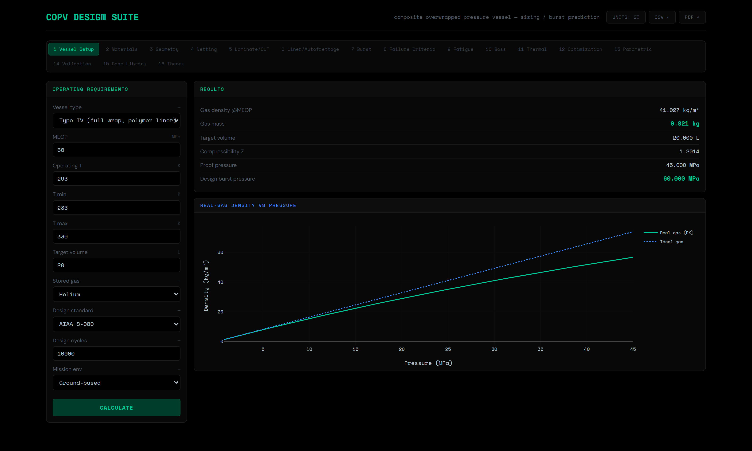
Solves the Redlich-Kwong equation of state via Brent root-finding for stored-gas molar volume at MEOP/temperature, giving density, compressibility factor Z, and required internal volume for a target stored mass — the ideal-gas law alone is off by several percent at typical 20–70 MPa pressurant conditions.
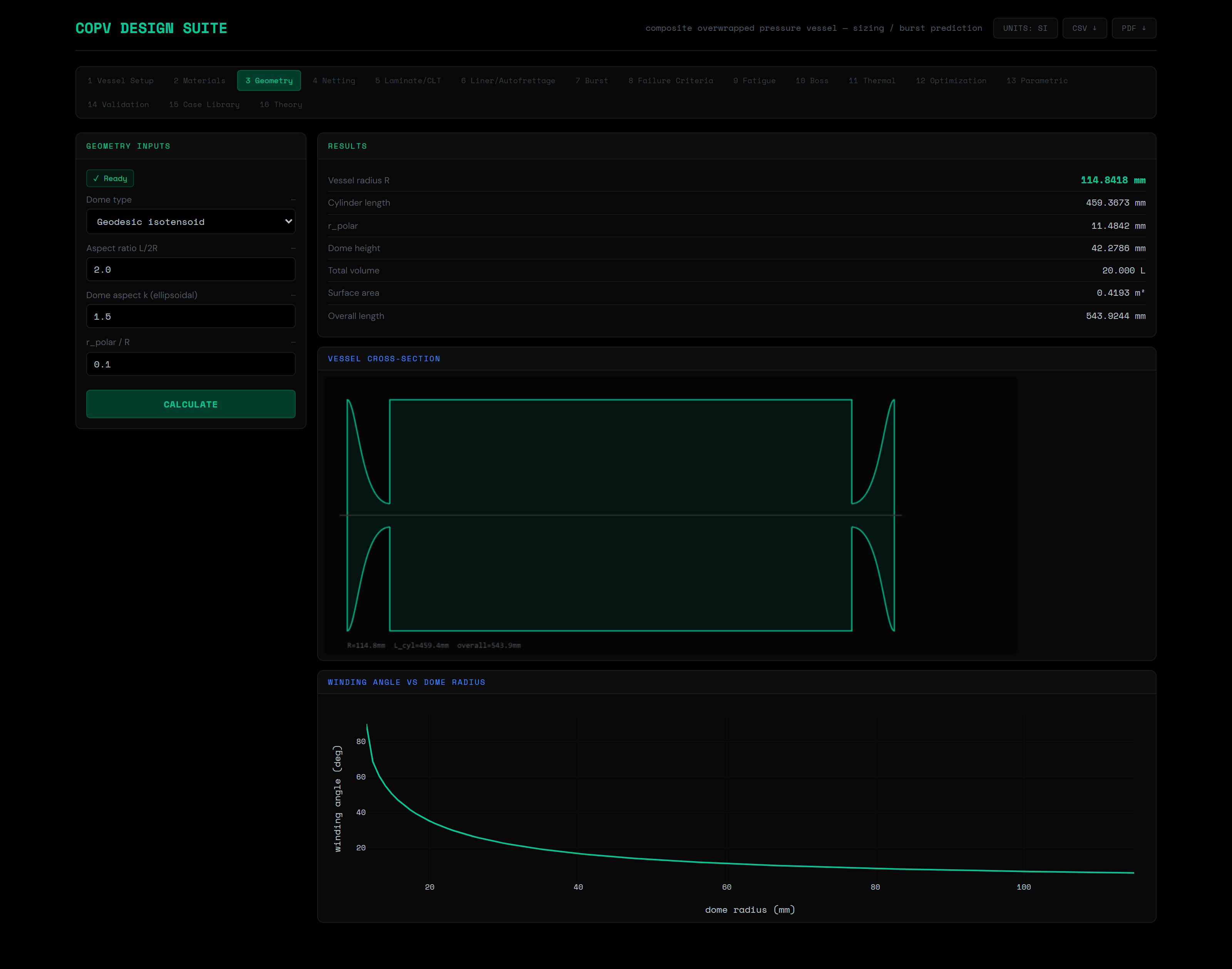
Hemispherical, ellipsoidal, torispherical (ASME F&D), and geodesic-isotensoid domes; volume/area via numerical revolution of the meridian, geodesic dome contour solved as an ODE via the r=R·sinθ substitution that removes both endpoint singularities.
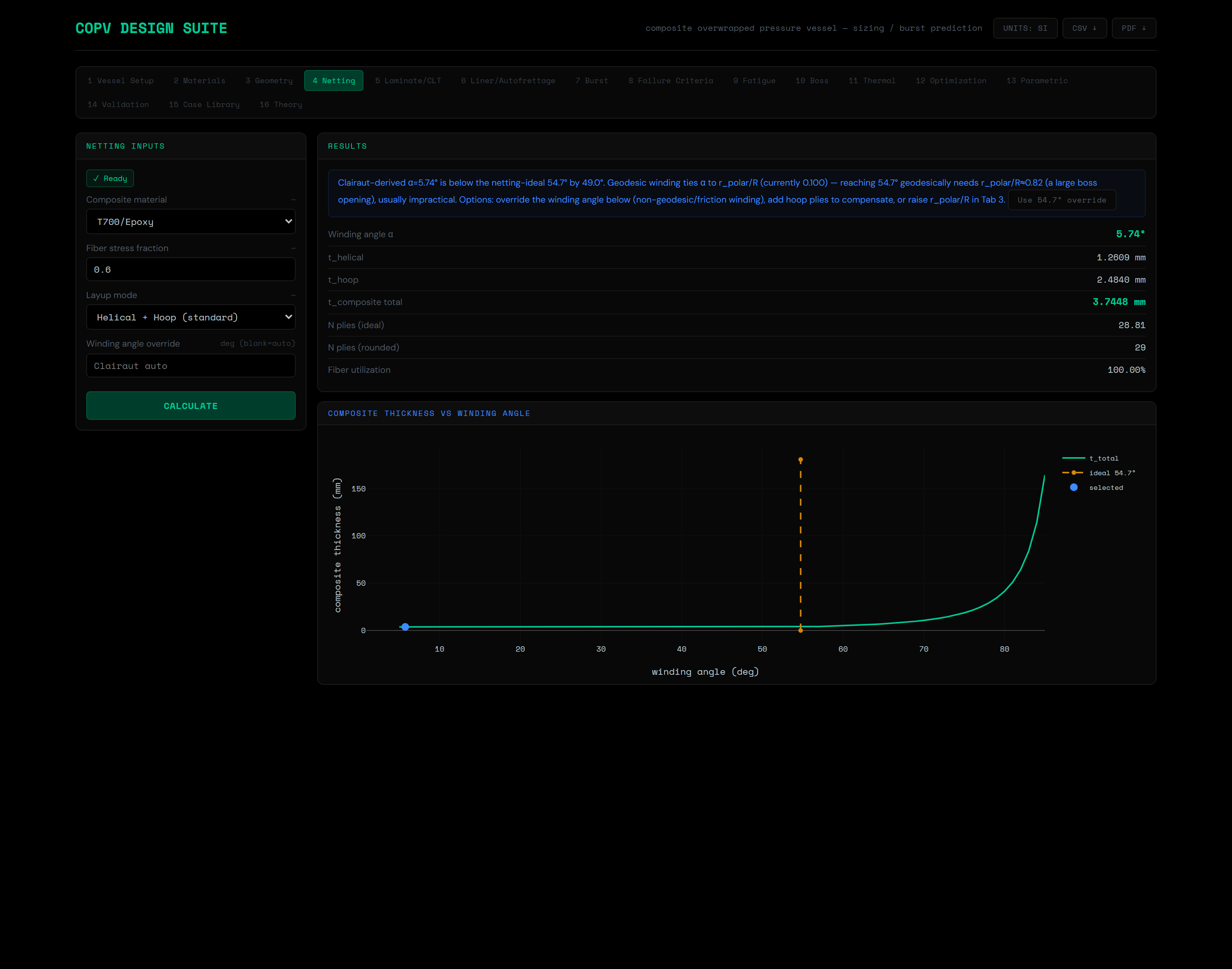
Solves helical/hoop ply thickness from fiber-only membrane equilibrium; flags the 54.7356° ideal angle where hoop-ply thickness first hits zero, with manufacturability checks on winding angle range.
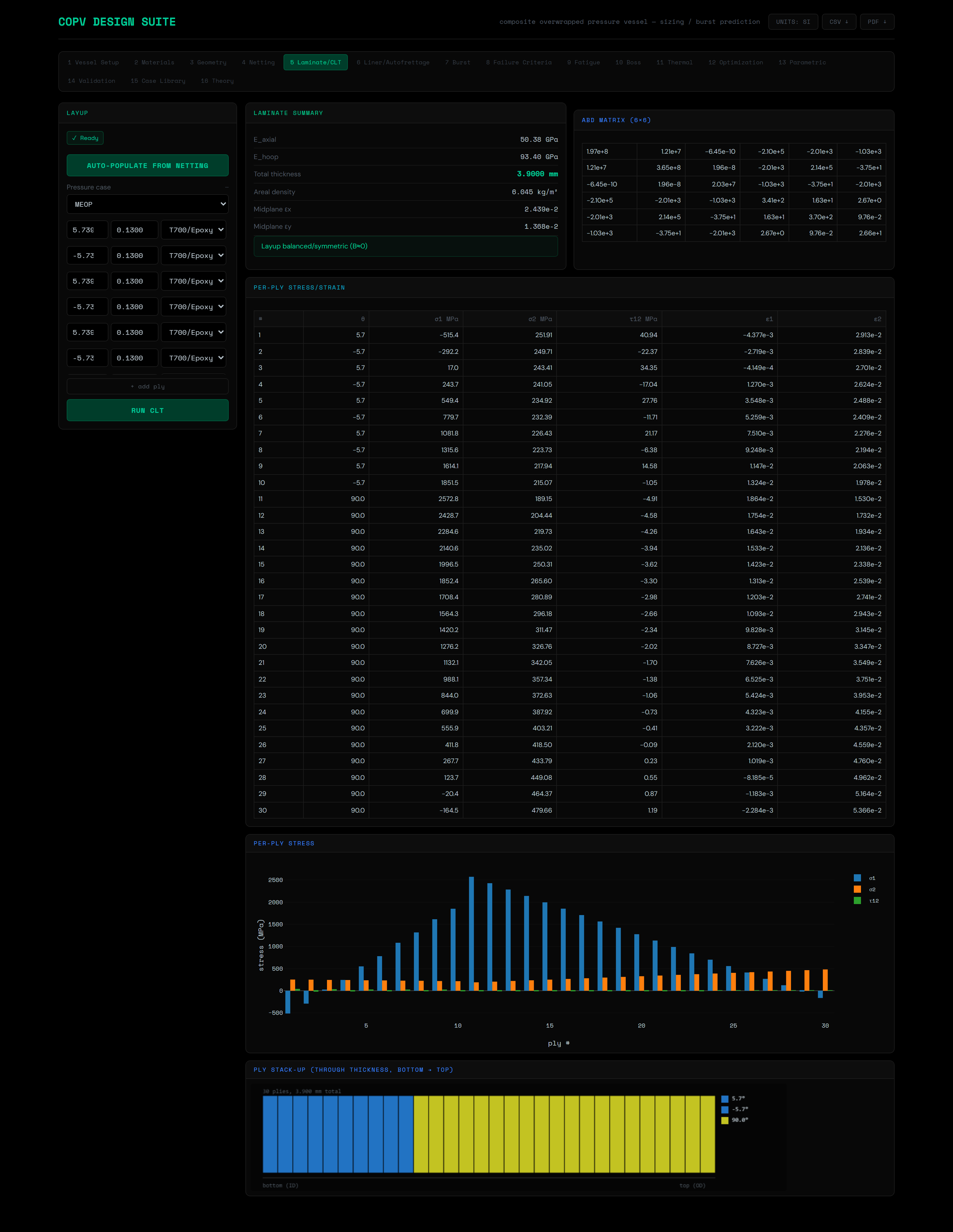
Auto-populates a symmetric [±α]n/[90]m stack from the netting result, assembles the ABD stiffness matrix from each ply's transformed reduced stiffness, solves midplane strain under the pressure-vessel membrane load, and recovers material-axis stress/strain in every ply — the ply-stacking canvas diagram shows the physical layup order.
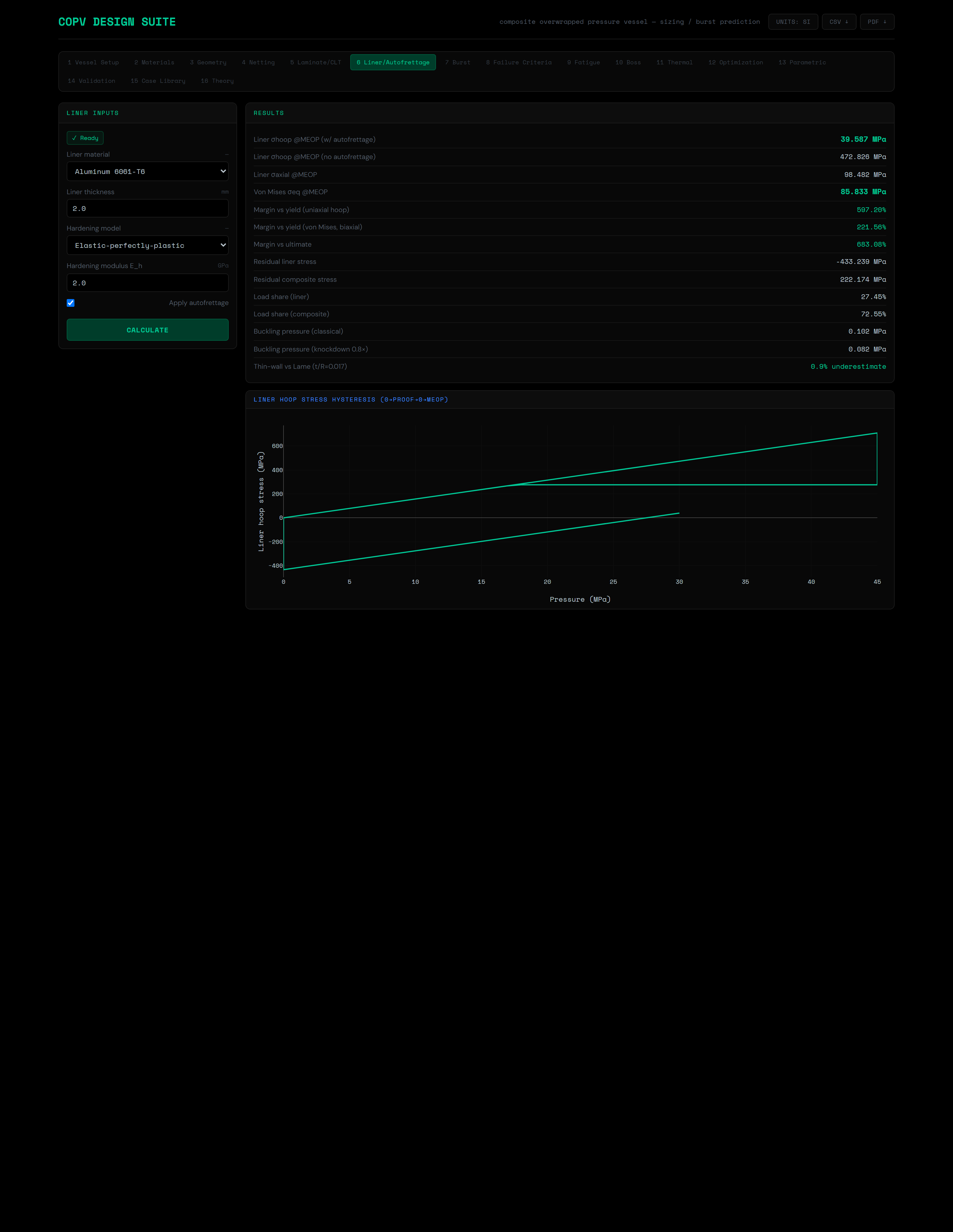
Strain-compatibility load sharing between liner and composite, elastic-plastic proof-cycle autofrettage (residual compressive liner stress), von Mises biaxial yield check, Lamé thick-wall cross-check, and NASA SP-8007-style external-pressure buckling knockdown.
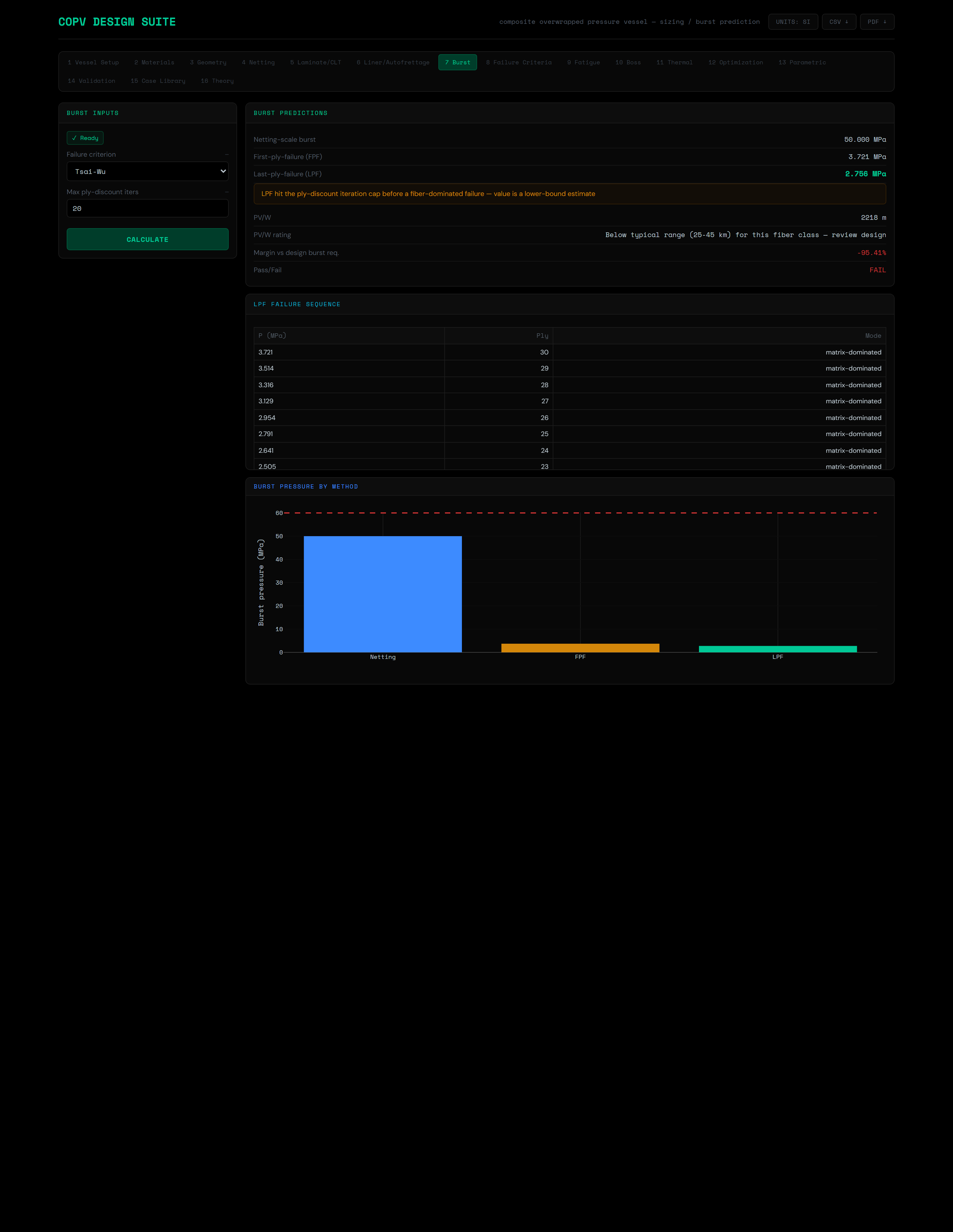
Netting-scale linear burst, first-ply-failure, progressive last-ply-failure (ply-discount "sudden death" degradation), and the PV/W historical flight-heritage performance correlation, side by side.
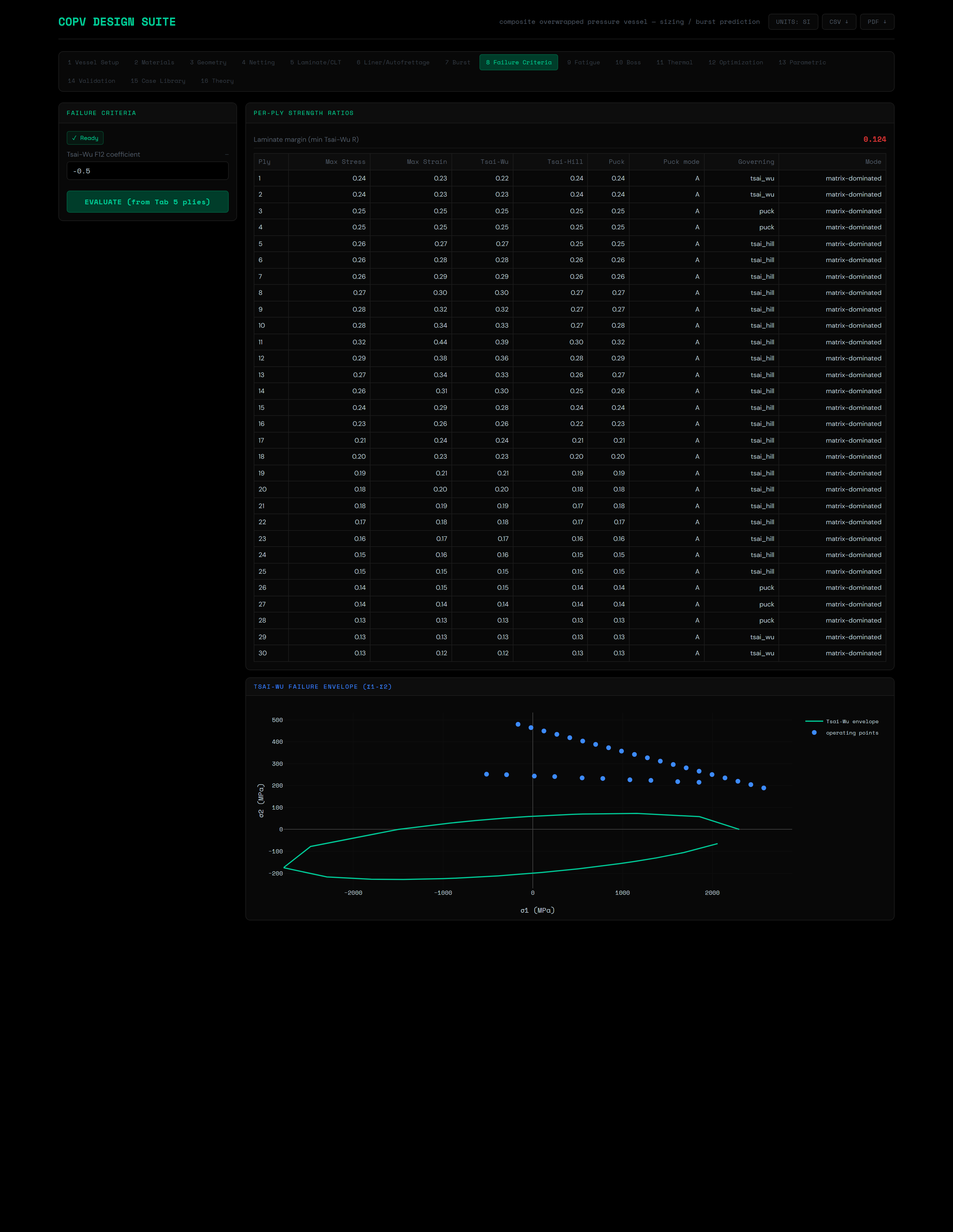
Max stress, max strain, Tsai-Wu (quadratic interaction surface), Tsai-Hill, and Puck (mode-resolved fiber/inter-fiber failure, action-plane theory) computed for every ply, with the governing criterion and failure mode surfaced per ply and an interactive Tsai-Wu envelope chart of the operating stress state.
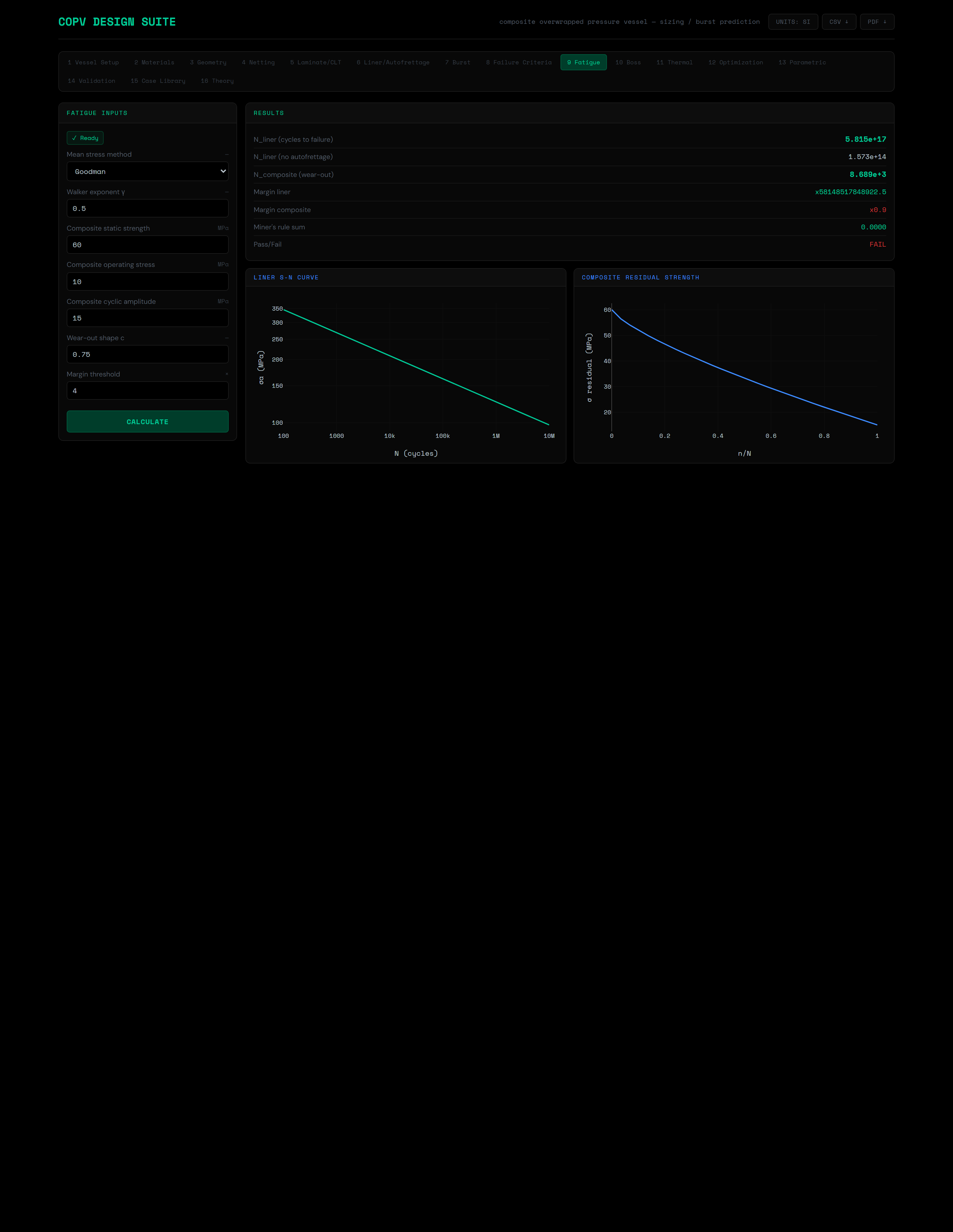
Basquin S-N liner metal fatigue with Goodman/Walker mean-stress correction, composite residual-strength wear-out degradation, and Miner's cumulative linear damage across the defined proof/MEOP cycle mix.
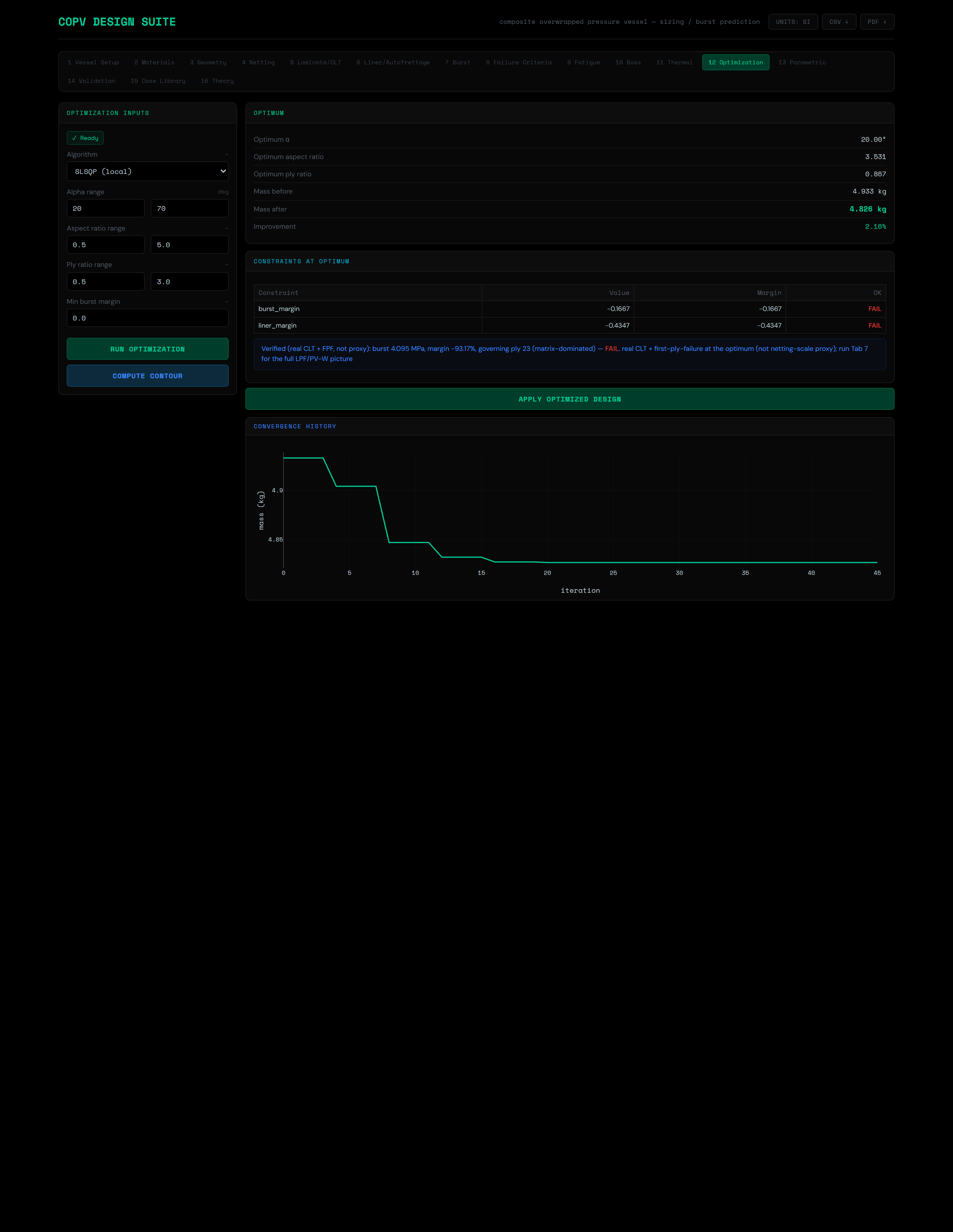
Minimizes vessel mass over winding angle, aspect ratio, and ply ratio subject to burst and liner-margin constraints using a fast proxy chain, then re-solves the real CLT + first-ply-failure chain at the reported optimum and shows both — this particular run shows the verification pass catching a proxy/reality mismatch (FAIL) rather than silently trusting the fast proxy, exactly the check it exists to make.
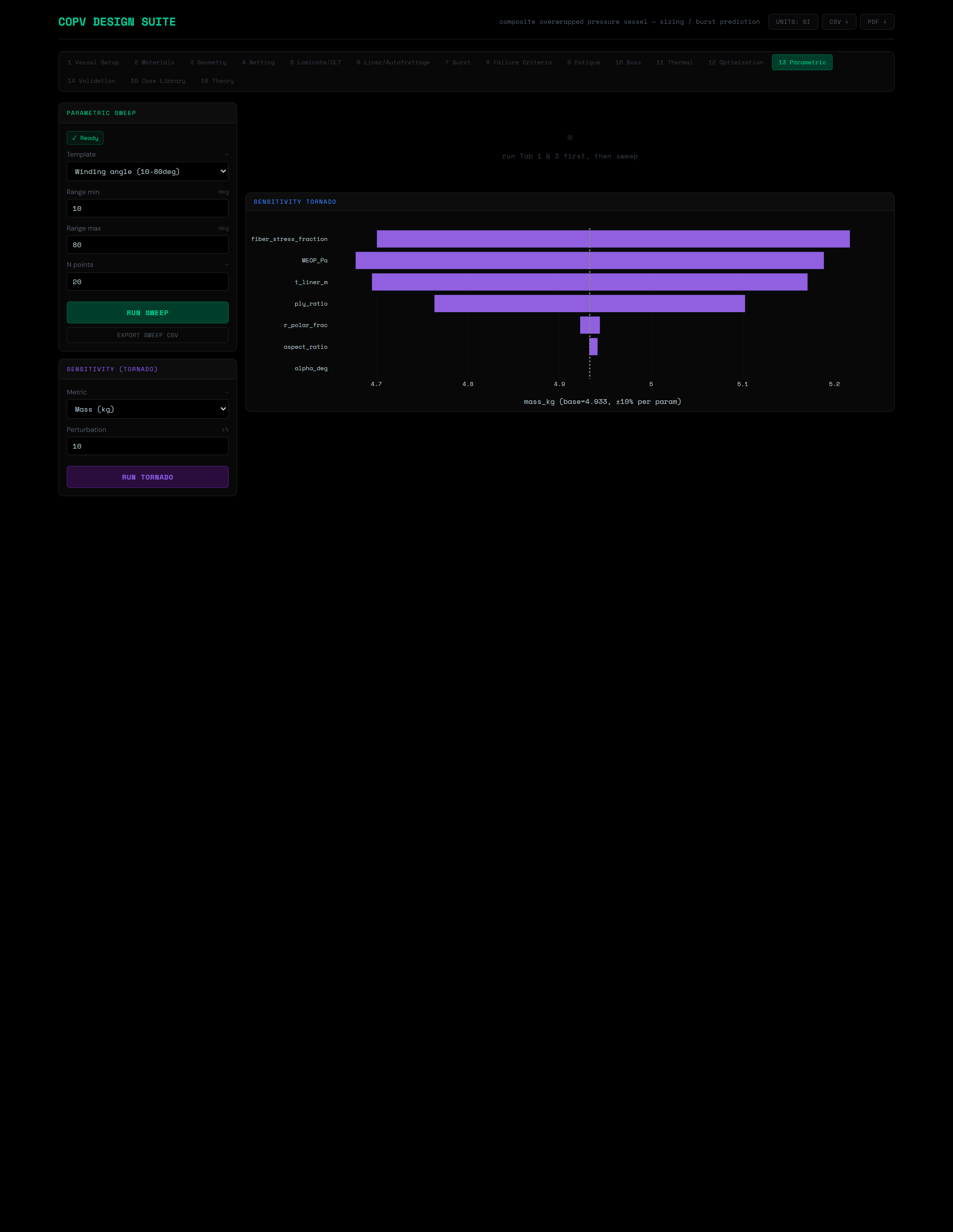
Perturbs α, aspect ratio, ply ratio, MEOP, rpolar/R, fiber-stress fraction, and liner thickness by ±10% around the current design and plots the resulting swing in mass or burst margin, sorted by magnitude.

Every physics module ships with at least one closed-form or self-consistency check — Barlow's formula, the 54.7356° ideal netting angle, Clairaut's relation, a balanced cross-ply CLT identity, Tsai-Wu at a defining strength point, autofrettage residual-stress sign, PV/W historical sanity band, real-gas Helium density, Puck's four uniaxial strength points, the von Mises equal-biaxial identity, the Lamé→thin-wall asymptotic limit, buckling-knockdown wiring, and a rule-of-mixtures modulus cross-check against published T700 fiber data. See the full breakdown in the Validation section below.
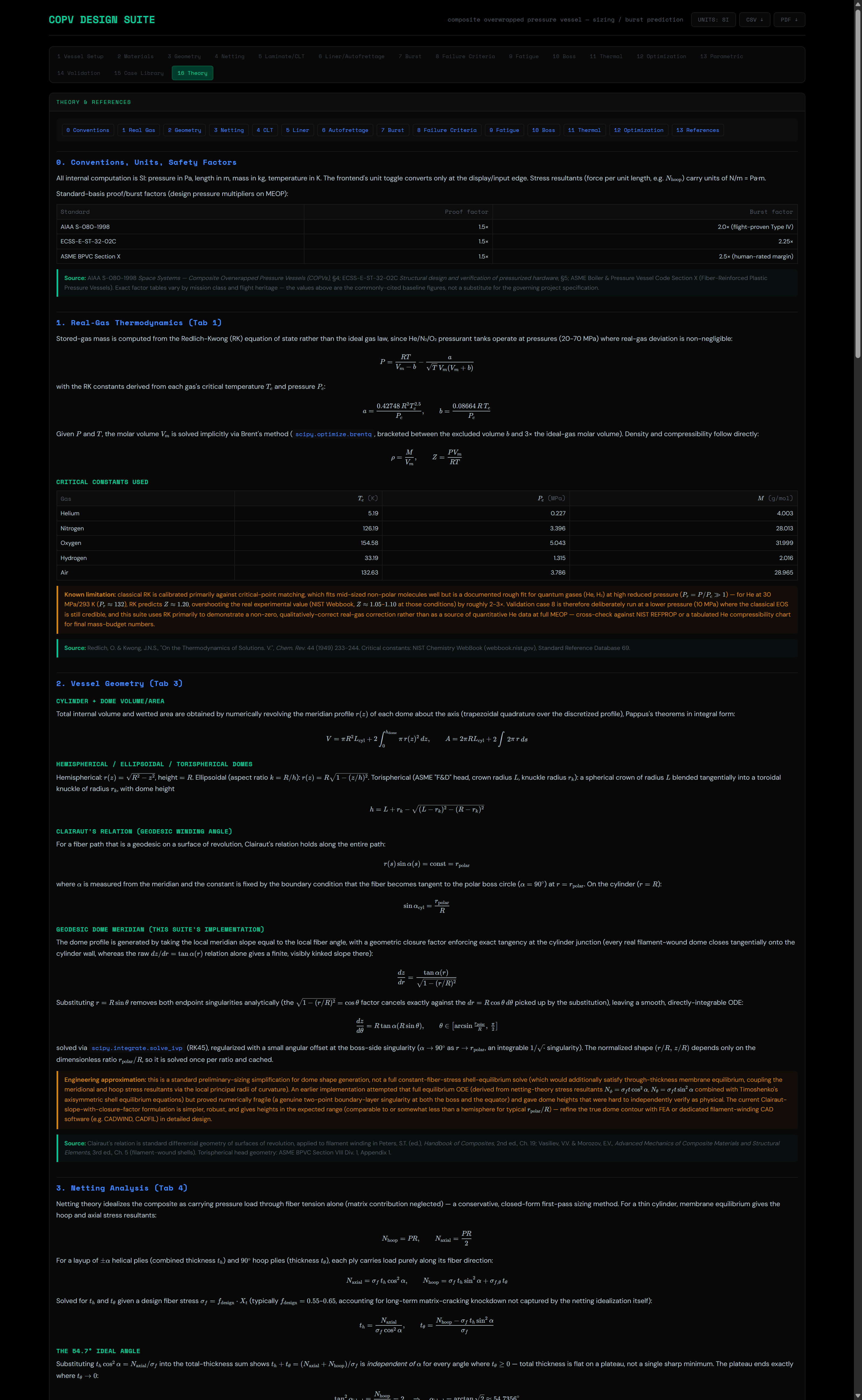
200+ KaTeX-rendered equations covering all 14 theory sections, each ending in a literature citation and, where a simplification is made, an explicit note on what it costs. The condensed version of this same content is in the Physics section of this page.
Condensed from the app's own Theory & References tab (Tab 16). Click a module to expand the governing equations, the derivation logic, and the literature it comes from.
All internal computation is SI (Pa, m, kg, K); the UI's unit toggle converts only at the display/input edge. Stress resultants (force per unit length) carry units N/m = Pa·m.
| Standard | Proof factor | Burst factor |
|---|---|---|
| AIAA S-080-1998 | 1.5× | 2.0× (flight-proven Type IV) |
| ECSS-E-ST-32-02C | 1.5× | 2.25× |
| ASME BPVC Section X | 1.5× | 2.5× (human-rated) |
Stored-gas mass uses the Redlich-Kwong equation of state, not the ideal gas law — at 20–70 MPa pressurant conditions the real-gas deviation is non-negligible:
$$ P = \frac{RT}{V_m - b} - \frac{a}{\sqrt{T}\, V_m (V_m + b)} $$
with constants from each gas's critical temperature/pressure:
$$ a = \frac{0.42748\, R^2 T_c^{2.5}}{P_c}, \qquad b = \frac{0.08664\, R\, T_c}{P_c} $$
Given P, T, the molar volume is solved implicitly via Brent's method
(scipy.optimize.brentq), then density and compressibility follow directly:
$$ \rho = \frac{M}{V_m}, \qquad Z = \frac{P V_m}{R T} $$
Volume/area from numerical revolution of the meridian (Pappus's theorems in integral form). For a fiber path that is a geodesic on a surface of revolution, Clairaut's relation holds along the entire path:
$$ r(s)\sin\alpha(s) = \text{const} = r_\text{polar}, \qquad \sin\alpha_\text{cyl} = \frac{r_\text{polar}}{R} $$
The dome meridian is generated from the local slope equal to the local fiber angle, with a closure factor enforcing exact tangency at the cylinder junction:
$$ \frac{dz}{dr} = \frac{\tan\alpha(r)}{\sqrt{1-(r/R)^2}} $$
Substituting $r=R\sin\theta$ removes both endpoint singularities analytically:
$$ \frac{dz}{d\theta} = R\tan\alpha(R\sin\theta), \qquad \theta \in \left[\arcsin\tfrac{r_\text{polar}}{R},\ \tfrac{\pi}{2}\right] $$
solved via scipy.integrate.solve_ivp (RK45), cached per rpolar/R ratio.
Fiber-only membrane equilibrium (matrix neglected — conservative first-pass sizing). Thin-cylinder resultants:
$$ N_\text{hoop} = PR, \qquad N_\text{axial} = \frac{PR}{2} $$
Solved for helical (±α) and hoop ply thickness at design fiber stress $\sigma_f = f_\text{design}\cdot X_t$:
$$ t_h = \frac{N_\text{axial}}{\sigma_f \cos^2\alpha}, \qquad t_\theta = \frac{N_\text{hoop} - \sigma_f\, t_h \sin^2\alpha}{\sigma_f} $$
Total thickness $t_h+t_\theta=(N_\text{axial}+N_\text{hoop})/\sigma_f$ is independent of α up to the angle where $t_\theta\to0$:
$$ \tan^2\alpha_\text{ideal} = \frac{N_\text{hoop}}{N_\text{axial}} = 2 \quad\Rightarrow\quad \alpha_\text{ideal} = \arctan\sqrt{2} \approx 54.7356^\circ $$
Beyond it, $t_\theta$ clamps to zero and $t_h$ alone must grow — validation case 2 confirms this transition numerically.
Reduced ply stiffness in material axes:
$$ Q_{11}=\frac{E_1}{1-\nu_{12}\nu_{21}},\ \ Q_{22}=\frac{E_2}{1-\nu_{12}\nu_{21}},\ \ Q_{12}=\frac{\nu_{12}E_2}{1-\nu_{12}\nu_{21}},\ \ Q_{66}=G_{12} $$
transformed to laminate axes via $[T]$ ($m=\cos\theta,\ n=\sin\theta$) and the Reuter matrix $[R]=\text{diag}(1,1,2)$:
$$ [\bar Q]_k = [T]^{-1}[Q]_k [R][T][R]^{-1} $$
ABD assembly over ply interface coordinates $z_{k-1},z_k$:
$$ A_{ij}=\sum_k [\bar Q_{ij}]_k(z_k-z_{k-1}),\quad B_{ij}=\frac12\sum_k [\bar Q_{ij}]_k(z_k^2-z_{k-1}^2),\quad D_{ij}=\frac13\sum_k [\bar Q_{ij}]_k(z_k^3-z_{k-1}^3) $$
Membrane solve for the pressure-vessel case ($M=0$):
$$ N = [A]\,\varepsilon^0, \qquad N = [N_\text{axial},\ N_\text{hoop},\ 0]^T $$
inverted for midplane strain, then per-ply stress from $[\sigma]_k=[Q]_k[\varepsilon]_k$ after rotating strain into material axes. Effective laminate moduli, back-calculated from A:
$$ E_x = \frac{A_{11}A_{22}-A_{12}^2}{A_{22}\, t}, \qquad E_y = \frac{A_{11}A_{22}-A_{12}^2}{A_{11}\, t} $$
Liner and composite as two bonded concentric thin cylinders, equal strain compatibility:
$$ \varepsilon = \frac{N}{E_\text{liner}t_\text{liner} + E_\text{composite}t_\text{composite}}, \qquad \sigma_\text{liner}=E_\text{liner}\varepsilon,\quad \sigma_\text{composite}=E_\text{composite}\varepsilon $$
In the liner-only limit this collapses exactly to Barlow's formula $\sigma_\text{hoop}=PR/t$ (validation case 1). Lamé thick-wall cross-check (inner radius a, outer b), maximized at the bore:
$$ \sigma_{\theta,\max} = \frac{P(a^2+b^2)}{b^2-a^2} $$
flagged once t/R ≥ 0.1 makes the thin-wall estimate meaningfully non-conservative (validation case 11 confirms convergence as t/R→0). Von Mises biaxial yield — the liner sees hoop and axial stress at once:
$$ \sigma_\text{vM} = \sqrt{\sigma_\text{hoop}^2 - \sigma_\text{hoop}\sigma_\text{axial} + \sigma_\text{axial}^2} $$
(equal-biaxial identity $\sigma_\text{vM}=\sigma$ exactly — validation case 10). External-pressure buckling, classical thin-shell (long-cylinder, n=2 lobe):
$$ P_{cr,\text{classical}} = \frac{E_\text{liner}}{4(1-\nu^2)}\left(\frac{t}{R}\right)^3, \qquad P_{cr} = \gamma_\text{ext}\, P_{cr,\text{classical}},\ \ \gamma_\text{ext}=0.8\ (\text{default}) $$
During proof pressure the liner can yield in hoop tension while the composite stays elastic; on depressurization the elastic composite springs back further than the now permanently-stretched liner, leaving the liner in residual compression (validation case 6 confirms the sign). Elastic-plastic proof strain:
$$ \varepsilon_\text{proof} = \frac{P_\text{proof}R - \sigma_y t_\text{liner} + E_h \varepsilon_y t_\text{liner}}{E_h t_\text{liner} + E_\text{composite}t_\text{composite}}, \qquad \varepsilon_y = \frac{\sigma_y}{E_\text{liner}} $$
Elastic unload to zero, then reload elastically to MEOP:
$$ \sigma_{\text{liner,res}} = E_\text{liner}(\varepsilon_\text{after unload}-\varepsilon_p), \qquad \sigma_\text{liner}(\text{MEOP}) = \sigma_{\text{liner,res}} + E_\text{liner}\cdot \frac{P_\text{MEOP}R}{E_\text{liner}t_\text{liner}+E_\text{composite}t_\text{composite}} $$
Netting-scale:
$$ P_{burst,\text{netting}} = P_\text{design}\cdot\frac{X_t}{\sigma_{f,\text{design}}} $$
First-ply-failure: since the CLT membrane response is linear in pressure for a fixed stiffness state, each ply's strength ratio at a reference pressure scales directly to its failure pressure:
$$ P_{burst,\text{FPF}} = P_\text{ref}\cdot\min_k R_k $$
Last-ply-failure (progressive ply-discount): after each matrix failure, that ply's transverse/shear stiffness is discounted (E2, G12→×10-6), the ABD matrix rebuilt, repeated until a fiber-dominated failure occurs — the true burst point.
PV/W historical correlation (sanity check, not predictive):
$$ \frac{PV}{W} = \frac{P_{burst}\cdot V_\text{internal}}{W_\text{composite}}, \qquad \left[\frac{PV}{W}\right]_\text{m} = \frac{PV/W}{g} $$
Typical flight-qualified bands: carbon/epoxy Type IV ≈ 25–45 km; aramid/epoxy ≈ 15–25 km.
Max stress/strain (no mode interaction):
$$ R = \min\left(\frac{X_{t/c}}{\sigma_1},\ \frac{Y_{t/c}}{\sigma_2},\ \frac{S}{|\tau_{12}|}\right) $$
Tsai-Wu (quadratic interaction surface):
$$ F_1\sigma_1+F_2\sigma_2+F_{11}\sigma_1^2+F_{22}\sigma_2^2+F_{66}\tau_{12}^2+ 2F_{12}\sigma_1\sigma_2 = 1, \qquad R = \frac{-b+\sqrt{b^2+4a}}{2a} $$
Tsai-Hill (anisotropic Hill-yield adaptation):
$$ \left(\frac{\sigma_1}{X}\right)^2 - \frac{\sigma_1\sigma_2}{X^2} + \left(\frac{\sigma_2}{Y}\right)^2 + \left(\frac{\tau_{12}}{S}\right)^2 = \frac1{R^2} $$
Puck (2D action-plane, mode-resolved fiber/inter-fiber failure) — Mode A (transverse tension + shear), Mode B (shear-dominated compression), Mode C (compression-dominated):
$$f_{E,A} = \sqrt{\left(\frac{\tau_{21}}{S}\right)^2 + \left(1-p_{\perp\parallel}^{+}\frac{Y_t}{S} \right)^2\left(\frac{\sigma_2}{Y_t}\right)^2} + p_{\perp\parallel}^{+}\frac{\sigma_2}{S}$$
$$f_{E,C} = \left[\left(\frac{\tau_{21}}{2(1+p_{\perp\perp}^{-})S}\right)^2 + \left(\frac{\sigma_2}{Y_c}\right)^2\right]\frac{Y_c}{-\sigma_2}, \qquad R_\text{Puck}=\min(R_{FF},R_{IFF})$$
Liner metal fatigue (Basquin):
$$ \sigma_a = \sigma_f'(2N)^b \quad\Rightarrow\quad N = \frac12\left(\frac{\sigma_a}{\sigma_f'}\right)^{1/b} $$
Mean-stress correction (Goodman or Walker):
$$ \sigma_{a,\text{eq}} = \frac{\sigma_a}{1-\sigma_m/\sigma_u}, \qquad \sigma_{a,\text{eq}} = \sigma_{\max}\left(\frac{1-R_\sigma}2\right)^{1-\gamma} $$
Composite residual-strength wear-out:
$$ \sigma_\text{residual}(n) = \sigma_\text{static} - (\sigma_\text{static}-\sigma_a) \left(\frac{n}{N}\right)^c $$
Miner's cumulative linear damage:
$$ \sum_i \frac{n_i}{N_i} \le 1 $$
Classical Volkersen shear-lag bondline load transfer near the boss:
$$ \tau(x) = \tau_{\max} e^{-x/\lambda}, \qquad \lambda = \left[\frac{G_a}{t_a}\left(\frac1{E_\text{boss}t_\text{boss}} + \frac1{E_\text{composite}t_\text{composite}}\right)\right]^{-1/2}, \qquad \tau_{\max} = \frac{N_\text{axial}}{\lambda} $$
Boss/composite CTE mismatch on cooldown (same stiffness-weighted compatibility structure as liner load-sharing, applied to free thermal strain):
$$ \varepsilon_\text{common} = \frac{(E_\text{boss}t_\text{boss}\alpha_\text{boss} + E_\text{composite}t_\text{composite}\alpha_\text{composite})\,\Delta T} {E_\text{boss}t_\text{boss}+E_\text{composite}t_\text{composite}} $$
CTE mismatch between differently-oriented plies generates residual stress on cooldown, handled by a thermal force/moment term added to the CLT balance:
$$ N^T = \sum_k [\bar Q]_k\,\vec\alpha_k\,\Delta T\,(z_k-z_{k-1}) $$
solved at $[N,M]=[N^T,M^T]$; mechanical (stress-producing) strain is total strain minus each ply's own free thermal strain. Permeation (informational, Type IV/V) via steady-state Fick's law:
$$ \dot n = \frac{\Phi \cdot A \cdot \Delta P}{t_\text{liner}} $$
Minimize vessel mass over winding angle, aspect ratio, and hoop:helical ply ratio, subject to burst-margin and liner-stress-margin constraints:
$$ \min_{\alpha,\ AR,\ r_\text{ply}}\ m(\alpha, AR, r_\text{ply}) \quad\text{s.t.}\quad \frac{P_{burst}}{P_{burst,\text{req}}}-1 \ge 0,\quad \frac{\sigma_y}{\sigma_\text{liner}}-1\ge0 $$
via scipy.optimize.minimize (SLSQP) or differential_evolution
(global, penalty-constrained). The search uses fast netting-scale/strain-compatibility
proxies for responsiveness; a one-shot verification pass then re-solves the real
netting→CLT→first-ply-failure chain at the reported optimum, surfacing any
proxy/reality mismatch rather than hiding it (see the Tab 12 screenshot above and the
Engineering Rigor section).
Every case is a closed-form textbook formula, a documented limiting/degenerate case, or a cross-check against a specific cited published constituent value — not a claim of matching unpublished proprietary test data. Re-run live under Tab 14 on every page load.
| # | Category | Check | Result |
|---|---|---|---|
| 1 | Liner Stress | Thin-wall hoop stress (Barlow's formula) — liner-only limit of the load-sharing solve reduces exactly to σ=PR/t | PASS |
| 2 | Netting Analysis | Ideal netting angle (54.7356°): hoop-ply thickness → 0 at it, total thickness strictly rises above it | PASS |
| 3 | Geometry | Clairaut relation at rpolar/R = 0.2 matches arcsin(0.2) analytically | PASS |
| 4 | Laminate Theory | Balanced cross-ply [0/90]s gives A11≈A22 (orthotropic symmetry identity) | PASS |
| 5 | Failure Criteria | Tsai-Wu strength ratio R≈1.0 at σ1=Xt (defining strength point) | PASS |
| 6 | Liner Stress | Autofrettage residual liner stress is compressive after proof-cycle yield (physical sign check) | PASS |
| 7 | Burst Prediction | PV/W sanity check for carbon/epoxy Type IV falls in the 20,000–50,000 m historical band | PASS |
| 8 | Gas Properties | Real-gas Helium density within 8% of ideal-gas at 10 MPa/293 K (near-ideal regime) | PASS |
| 9 | Failure Criteria | Puck IFF criterion at Yt/−Yc/S uniaxial points — R=1.0 in modes A/C/A respectively | PASS |
| 10 | Liner Stress | Von Mises equal-biaxial identity: σvM = σ exactly when hoop = axial | PASS |
| 11 | Liner Stress | Lamé thick-wall solution converges to thin-wall (Barlow) as t/R → 0 (<0.5% at t/R=0.001) | PASS |
| 12 | Liner Stress | Buckling knockdown pressure = k × classical pressure, exactly (wiring check) | PASS |
| 13 | Laminate Theory | Rule-of-mixtures E1 cross-check vs. Toray T700S published fiber modulus (within 10%) | PASS |
Backed by 11 pytest unit/integration tests (API smoke tests across all 16 routers, 4 dedicated
Puck mode-boundary tests, 1 full validation-suite assertion) — run with
pytest tests/ -v.
A validated model is worth more than a green checkmark. Two genuine physics-correctness bugs surfaced during development of this suite; both are documented here in full rather than quietly patched, because the process of catching them is itself the strongest evidence the final numbers can be trusted.
The initial implementation classified Puck's inter-fiber-failure Mode B (shear-dominated) vs. Mode C (compression-dominated) with the boundary inequality flipped. Caught by systematically evaluating all four uniaxial strength-defining stress states (Xt, Yt, −Yc, S) and checking each gives strength ratio R≈1.0 in its expected mode.
Fix: flipped the |σ2/τ21| transition-ratio comparison from ≥ to ≤. Now locked in permanently by validation case 9.
The liner's biaxial yield check combined a hoop stress that had gone through the autofrettage elastic-plastic solve with an axial stress computed by plain linear elasticity (no autofrettage) — an internally inconsistent combination. Caught not by any unit test, but by visually inspecting a live-browser screenshot of Tab 6 and noticing the margins didn't make physical sense together.
Fix: the axial direction now runs through the identical autofrettage solve as hoop (reusing it via a R→R/2 substitution, since the solver only ever uses R through the product P·R). Now locked in by validation case 10 and documented as a limitation (independent uniaxial solves per direction, not full coupled biaxial plasticity) in the theory tab.
Both fixes were confirmed three ways: direct Python sanity checks, the full pytest suite (11/11), and a live headless-Chrome walkthrough of the affected tabs with the numeric result inspected against expectation — the same class of check that caught them in the first place.
Every preliminary-design tool trades fidelity for speed somewhere. These are the specific places this one does, stated plainly rather than buried in a caveat nobody reads.
The dome contour comes from enforcing the local Clairaut winding-angle slope with a tangency-closure factor at the cylinder junction — not a full constant-fiber-stress through-thickness shell equilibrium (which would additionally couple meridional and hoop stress resultants via local curvature). A full-equilibrium ODE was attempted first and proved numerically fragile at both the boss and equator boundary layers. Refine with FEA or dedicated filament-winding CAD (CADWIND, CADFIL) for detailed design.
SLSQP/differential evolution use netting-scale burst margin and strain-compatibility liner margin as fast constraint proxies so the search stays responsive at hundreds of evaluations. The one-shot verification pass at the reported optimum runs the real CLT + first-ply-failure chain and is always shown alongside — a proxy/verified mismatch is a signal to widen the search bounds or check Tab 7 directly, not a hidden failure mode.
Laminates with many near-identical ply-angle groups (e.g. pure-helical layups with no distinguishing angles) can hit the iteration cap before reaching a fiber-dominated failure. The UI flags this explicitly and reports the last-found ratio as a lower-bound estimate, rather than silently presenting a capped value as converged.
Helium and hydrogen at high P/Pc deviate from RK's prediction by 2–3× the true compressibility correction (still small in absolute terms, but non-negligible for precision mass budgets). Cross-check against NIST REFPROP or a tabulated compressibility chart before finalizing pressurant mass at full MEOP.
Hoop and axial liner stress each go through the same autofrettage history independently, then combine via von Mises for the final yield check — not a single coupled biaxial flow-rule plasticity solution, which would let yielding in one direction affect the available strength in the other during the plastic proof-load excursion itself.
NASA SP-8007's empirical knockdown curve is derived for axial compression; external/hydrostatic pressure buckling is documented to be substantially less imperfection-sensitive, so a fixed γ=0.8 (user-overridable) stands in for the full curve as a representative preliminary-design factor.
Every equation in this suite traces to one of these — no formula was invented or approximated without a documented source.