Space systems · RVCE EL · 2024–25

CubeSat system for microplastic hotspots

Dual 6U constellation · X-band SAR + VNIR/SWIR · Sentinel-1/2 prototype
Experiential Learning (CV242TA), with Sanskar Verma, Sarthak Sharma, and Shambhavi Shukla. Guide: Dr. A R Vinod.

Two 6U CubeSats in the same sun-synchronous plane. One finds the slick on radar. The other stares at it in VNIR and SWIR. Ship sampling cannot map five trillion particles; this is the space-based try.

2 × 6Uconstellation
500–550 kmSSO
8.68 dBISL margin
simulatedpolymer labels

CubeSat 1 flies X-band SAR and flags patches of ocean where capillary waves are damped — the Mean Square Slope drop that slicks leave behind. CubeSat 2 takes those coordinates, images in VNIR and SWIR, and downlinks a classification map.

It is a concept plus a ground prototype, not a flown spacecraft. The flight architecture, antenna sizing, Sentinel scenes, fusion pipeline, and orbit animation are real work from the report. Polymer class labels from the detector are a prototype — the code itself treats type assignment as simulated.

STK / Ansys orbit view of the pair in a polar SSO, with in-track spacing and an S-band crosslink. Compressed from the original 48 s visualization.

Mission architecture

Orbit	Sun-synchronous, 500–550 km. In-track spacing 100–300 km.
CubeSat 1 — SAR	6U. X-band SAR at 9.6 GHz, ~100–200 MHz bandwidth, stripmap, ~10–15 m resolution, ~30 km swath. Role: MSS anomaly detection. Sends 1–10 KB metadata packets over S-band ISL.
CubeSat 2 — HSI	6U. VNIR CCD (400–1000 nm) and SWIR InGaAs (1000–2500 nm). Target bands: PET 1610 nm, PE 1730 nm, PP 2300 nm. ~30–50 m/pixel, 3–5 km swath. X-band downlink 10–20 Mbps.
Onboard SAR chain	Zynq-7020: range compression, Doppler azimuth compression, GPS/IMU motion compensation → 500×500 backscatter patch → 2D FFT to S(k) → MSS vs Hwang LUT. Flag if MSS drops more than 15%.

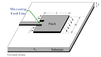
S-band patch for the crosslink

ISL is a 2.2 GHz S-band microstrip patch, 1 W, 8 dBi on each end, 200 km design range. Link budget in the report: FSPL 145.32 dB, received −101.32 dBm, margin 8.68 dB against −110 dBm.

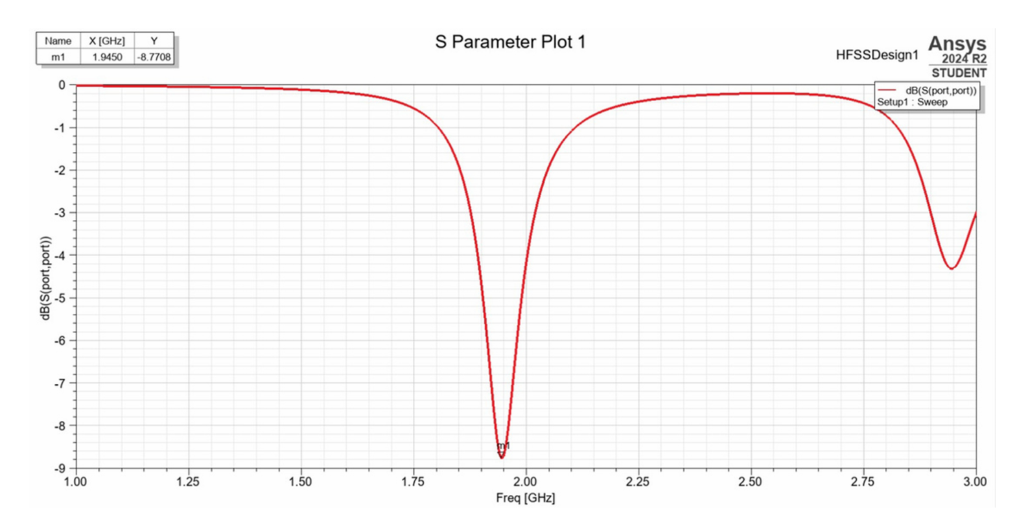
The sized patch uses RT/Duroid 6006 (ε_r = 6.0, tan δ = 0.0019, h = 3.2 mm). Closed-form dimensions at 2 GHz: W = 40.09 mm, L = 29.8 mm, substrate 59.3 × 49.0 mm. HFSS resonated at 1.945 GHz. Repeating the same method at 2.2 GHz gives 53.90 × 45.32 mm on a thinner 1.6 mm, ε_r = 2.2 stack. X-band SAR patch (9.6 GHz): 12.35 × 9.53 mm.

Microstrip patch antenna with feed line — Microstrip patch, feed, and substrate stack used for the ISL sizing.

HFSS S11 plot resonating at 1.945 GHz — HFSS S₁₁: resonance at 1.945 GHz, −8.77 dB. Close to the 2 GHz design point; 2.2 GHz is a retune, not a new topology.

Sentinel-1 and Sentinel-2 scenes

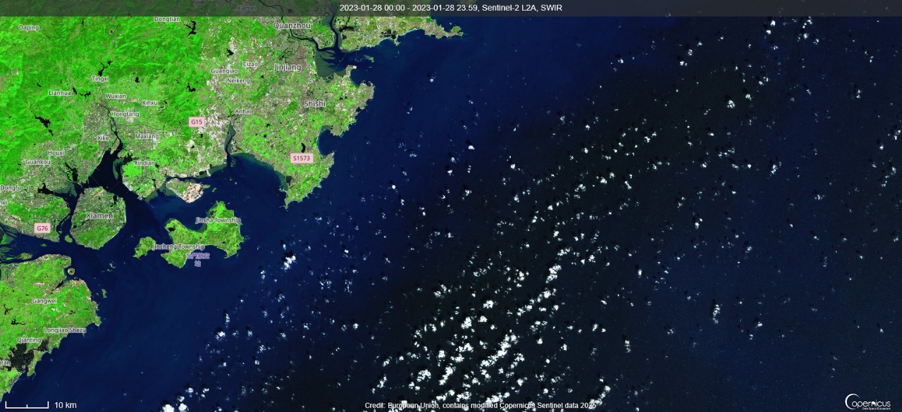
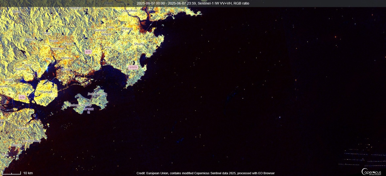
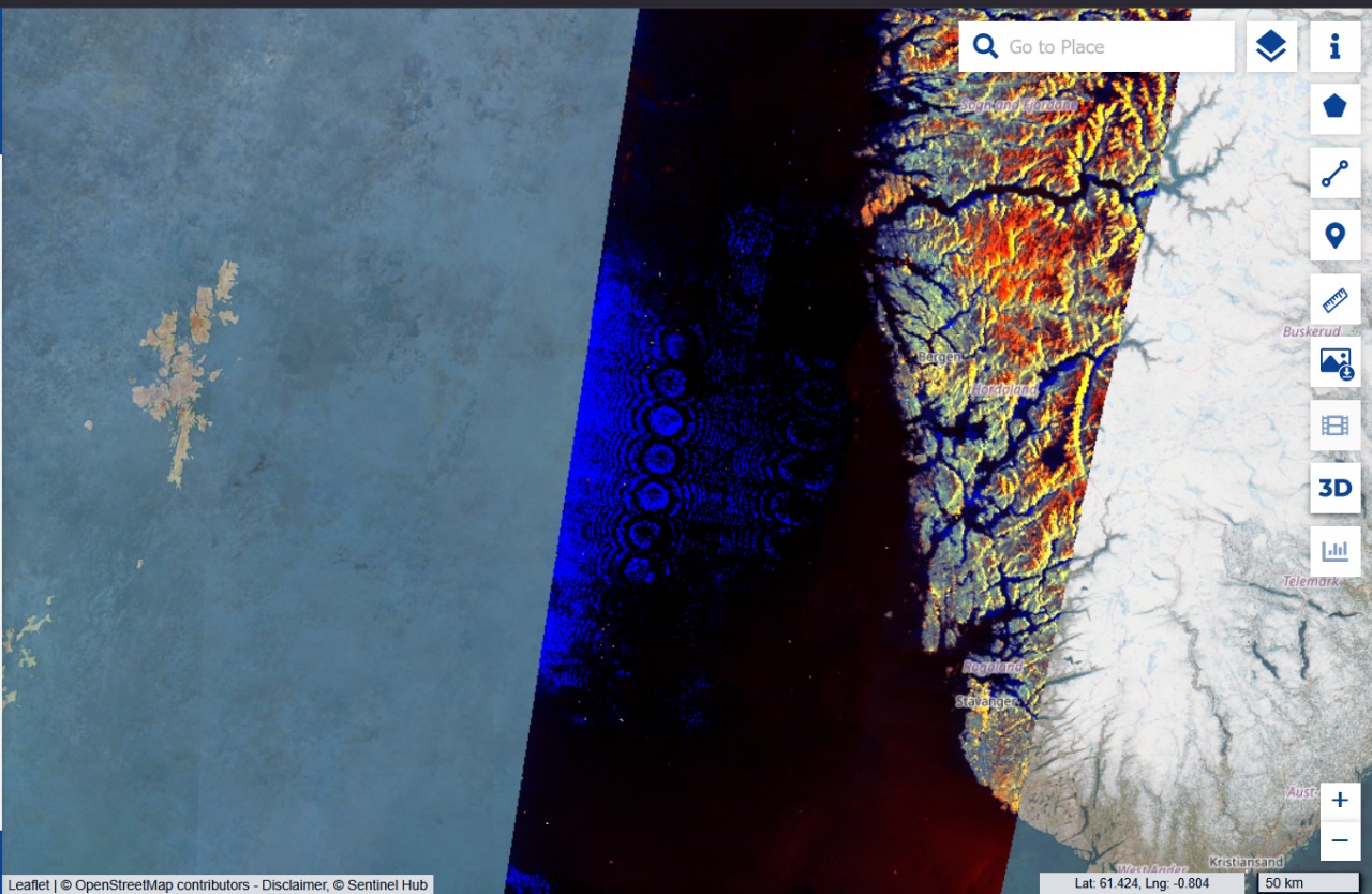
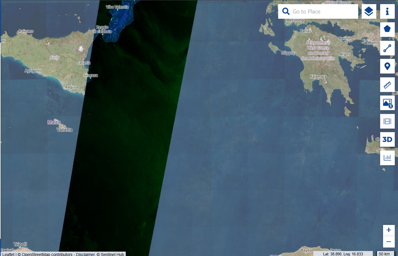
Before a CubeSat exists, the sensing idea has to run on public radar and optical. We pulled Sentinel-1 SAR and Sentinel-2 SWIR/RGB for three basins: South China Sea (industrial dumping along the Fujian coast, 28 Jan 2023), the Norwegian Sea off Bergen, and the central Mediterranean between Sicily and Greece.

Sentinel-2 SWIR of the South China Sea near Xiamen — South China Sea, Sentinel-2 L2A SWIR. Quanzhou–Xiamen coast.

South China Sea RGB ratio composite — Same region, RGB-ratio composite used in the fusion stack.

Sentinel-1 SAR over the Norwegian coast — Norway, Sentinel-1 SAR overlay on the coast near Bergen / Hordaland.

Sentinel-2 SWIR over the central Mediterranean — Mediterranean SWIR strip, Sicily–Malta–Greece.

Fusion on the ground

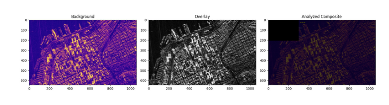
The Python fusion tool blends a SAR background with an optical overlay (ORB + brute-force matching, Laplacian variance for noise, Canny edges). On the South China Sea pair: blue channel dominant (R 97.7, G 36.2, B 138.3), 356 matched keypoints, Laplacian variance 1298.89, contrast 43.52.

SAR and optical fusion composite with technical overlay — Background / overlay / analyzed composite. The black box is the on-image analysis strip from the script.

Detection prototype

A second script, SatellitePlasticDetector, takes those scenes, builds Plastic Index / NDPI / FDI, thresholds the top 15% of the index, and draws connected patches. It then assigns PET, PE, PP, PS, or mixed debris. That last step is simulated — type is not a trained spectral library. Treat the boxes as “this is where the index fired,” not as laboratory polymer ID.

Norway SAR plastic detection dashboard — Norway SAR run: two PET-tagged patches, 0.3752 km² combined, confidence 0.85–0.95.

Mediterranean SWIR plastic detection dashboard — Mediterranean SWIR: PE/PP boxes along the Sentinel strip, 0.1492 km².

Mediterranean urban SAR detection dashboard — Mediterranean urban SAR: more boxes, 31.45 km² tagged — the large area is the whole strip firing, which is a limit of the threshold method, not a 31 km² slick.

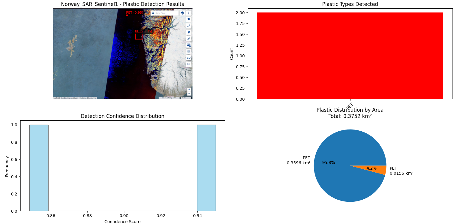
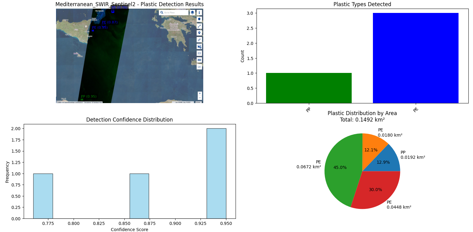
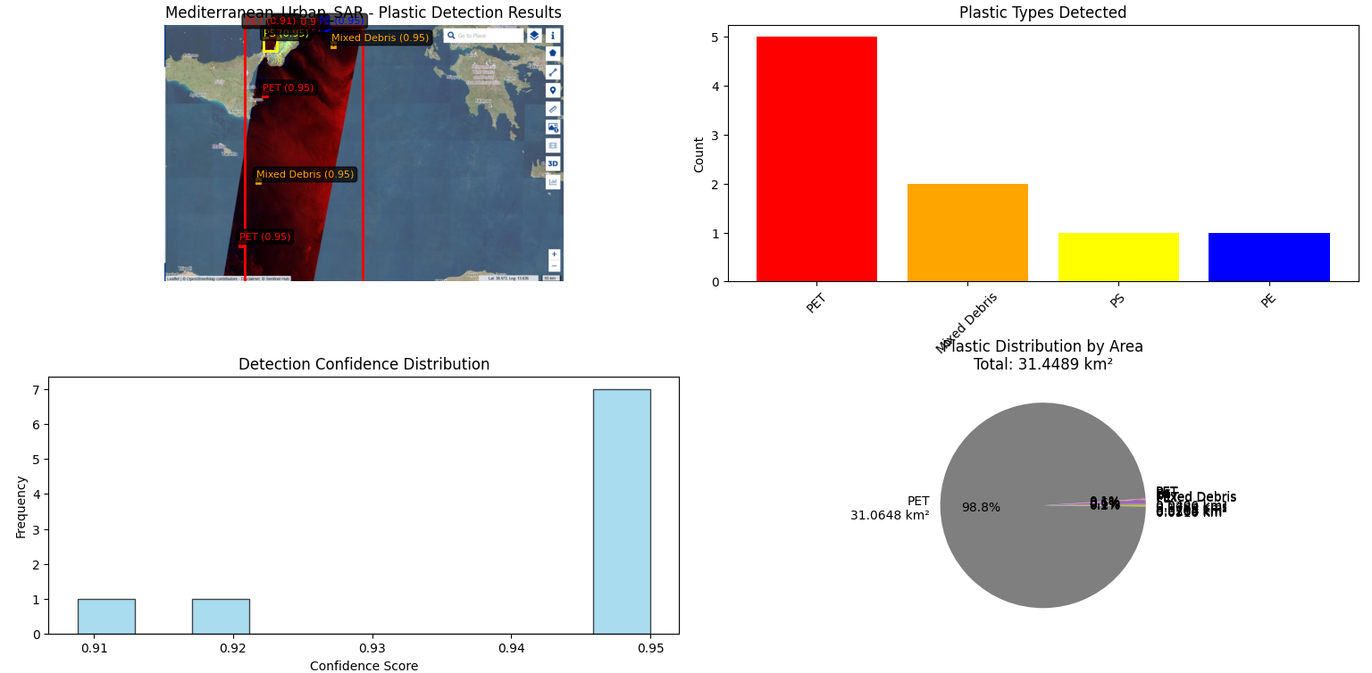
The useful part of this pipeline is the SAR→coordinate→optical cueing idea and the fact that it runs on real Copernicus scenes. A flown mission would replace the random type step with an onboard FNN on actual VNIR/SWIR cubes, which is what the architecture section specifies (SNV, Savitzky–Golay, mean-center, GeoTIFF out, 50–200 KB per scene).

Data path, in one line

SAR images → MSS vs LUT → hotspot packet (lat, lon, ΔMSS, confidence, CRC32, ~30–40 B) → S-band ISL → HSI queue (ephemeris + sun angle) → VNIR/SWIR cube → classify → X-band GeoTIFF to the ground, 4–6 passes/day, ~30–60 MB/day.

← Projects