Numerical Modeling of Electromagnetic Scattering
for Radar Cross Section Prediction
Overview
A first-principles computational framework (Python) integrating Physical Optics (PO), the Physical Theory of Diffraction (PTD), multi-bounce ray tracing (double/triple-bounce), Radar Absorbent Material (RAM) models including a Surface Impedance Boundary Condition (SIBC), bistatic/polarimetric extensions, a gradient-free geometry optimizer, wideband impulse response, validated against the exact Mie series.
1 Why Radar Cross Section Matters
What it is. RCS (
Why engineers track it in dBsm, not m2. Real targets span an enormous dynamic range, from a
stealth aircraft's fractional-square-metre nose-on return to a large cargo ship's tens-of-thousands of
square metres. Working in decibels relative to one square metre (dBsm
Why it drives detection range, not just "how visible" qualitatively. Substituting
Reference points, so the numbers on this site have context. F-15 Eagle (a conventional 1970s-era fighter shape, flat panels, right-angle intersections everywhere): frontal RCS roughly +10 to +14 dBsm (around 10–25 m2, comparable to a small truck). B-2 Spirit (a purpose-shaped stealth flying wing): frontal RCS roughly −20 to −30 dBsm (around 0.001–0.01 m2, comparable to a large bird or a golf ball). That is a >40 dB spread, a factor of 10,000× in raw reflected power, achieved almost entirely through shape, not stealth coatings alone. This project reproduces that same shaping mechanism at a smaller, teaching-scale level between its own "conventional" and "stealth" geometries.
2 Problem Statement
Aircraft are, first and foremost, designed to fly: their outer mould line is set by aerodynamics, structural load paths, internal volume for fuel, avionics, weapons, and manufacturing cost, radar visibility is historically an afterthought bolted on at the end (radar-absorbent paint, for instance). The consequence is that almost every conventional airframe accidentally contains near-ideal radar reflectors: a vertical tail is a large flat plate; a wing root is a right-angle dihedral; an engine inlet is a deep cavity with a spinning metal fan at the back of it. Modern low-observable ("stealth") design instead treats radar return as a first-class design constraint from day one, and achieves its reduction primarily through geometric shaping that redirects scattered energy away from the threat radar, with radar-absorbent material as a secondary, supporting layer. Reproducing and quantifying that shaping effect computationally runs into three concrete challenges:
- Challenge 1, coherent, not additive, physics. A real target's echo is the vector (complex, phase-carrying) sum of many simultaneous physical mechanisms: specular glint off flat panels (PO), diffraction that "leaks" around sharp edges (PTD), and re-reflection inside corners (multi-bounce). Adding their powers independently is a common shortcut in simplified tools, but it is physically wrong, two mechanisms can constructively or destructively interfere depending on relative phase, and only a fully coherent complex-amplitude sum captures that. This project sums complex amplitudes at every step and squares only at the very end.
- Challenge 2, strong non-linearity. RCS is not a smooth, gently-varying function of aspect angle. A one-degree rotation can swing the return by 20+ dB if it crosses a specular glint angle or activates/deactivates a corner-reflector pair. This makes the problem numerically stiff and rules out naive coarse angular sampling.
- Challenge 3, attribution, not just a number. Knowing "the RCS at 45° is 55 dBsm" is far less useful to a design engineer than knowing which panel or edge produced that 55 dBsm, so it can be reshaped. This project's mechanism-breakdown tab exists specifically to answer that attribution question quantitatively rather than by inspection or intuition.
3 Objectives
The core objective is to build the whole RCS-prediction pipeline from first principles, no commercial EM solver, no black-box RCS library, so every number on this site can be traced back to a specific equation and a specific line of Python. Concretely, the project set out to:
- Design a first-principles RCS framework in Python integrating PO, PTD, double/triple-bounce, and RAM models, so the same codebase can answer "what does this shape return" for any of the six test geometries.
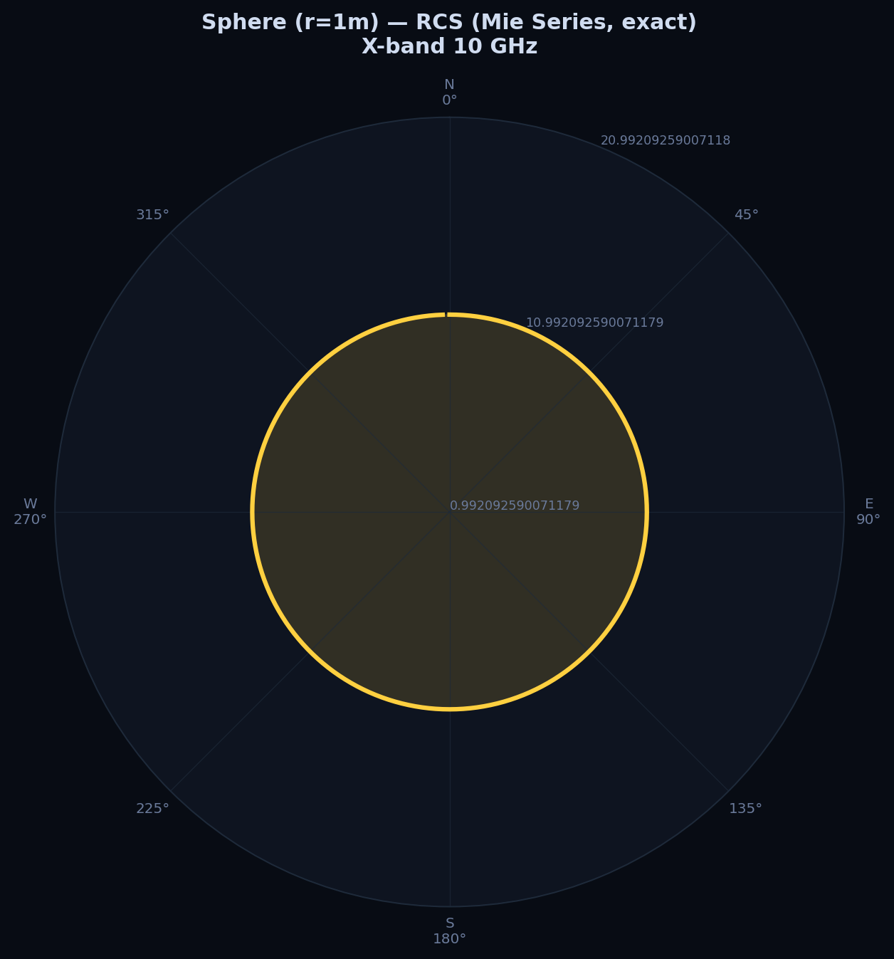
- Validate the PO solver against the exact Mie series for a conducting sphere, the one canonical shape electromagnetics has a closed-form exact answer for, and therefore the only fair, no-excuses correctness test.
- Analyse RCS of six triangulated-mesh geometries across azimuth, elevation, and frequency, rather than at a single "hero" angle that could hide unfavourable behaviour elsewhere.
- Evaluate dominant scattering mechanisms and derive low-observable design principles that a working aerospace engineer could actually apply to a new design, not just descriptive statistics about this one pair of shapes.
- Surface Impedance Boundary Condition for real finite-conductivity materials, a gradient-free geometry optimizer that searches for a better stealth shape automatically, wideband time-domain impulse response each accompanied by its own mesh-convergence study, because a result nobody has checked for mesh-independence is not yet a trustworthy result.
4 Background, Primary Scattering Contributors
Before building any solver, it is worth simply listing, in plain engineering terms, where most of a conventional aircraft's radar return actually comes from. None of these numbers require simulation, they are well-known rule-of-thumb figures from the RCS literature (Knott, Shaeffer & Tuley) for isolated canonical shapes at the aircraft's approximate real-world dimensions, and they motivate exactly which mechanisms this project needed to model.
| Feature | Geometry | Approx. RCS (X-band) |
|---|---|---|
| Vertical stabiliser (3×2 m) | Flat-plate broadside | ~+57 dBsm |
| Cylindrical fuselage (d=1.5 m, L=15 m) | Cylinder broadside | ~+42.5 dBsm |
| Unshielded engine inlet | Deep cavity retroreflector | +15 to +25 dBsm |
| Wing–fuselage junction | Dihedral corner reflector | +10 to +20 dBsm |
| Canopy / cockpit | Cavity, forward aspect | +5 to +15 dBsm |
Governing Physics & Scattering Mechanisms
Every RCS number in this project is a coherent complex-amplitude sum of three physical mechanisms,
squared at the end, never added as independent powers.
1 What is a Facet, and Why Mesh the Aircraft at All?
What. Every aircraft surface here is discretized into flat triangular facets, the same
faceted-mesh representation used in real RCS prediction codes (XPATCH, POFACETS, FEKO's PO solver). Each facet
Why not solve Maxwell's equations exactly on the real curved surface? Because an exact solution
(the Method of Moments, MoM) requires solving a dense linear system with one unknown per roughly
How illumination is decided. PO sums a phased contribution from every illuminated facet
(
2 Physical Optics (PO), Specular Reflection
What it models. The dominant "mirror-like" glint you get when a flat (or locally-flat) surface happens to be oriented so the incident ray reflects straight back at the radar. This is the single largest RCS contributor for almost any aircraft at almost any aspect, it is why a vertical tail fin lights up like a beacon at broadside and why a curved fuselage still returns a bright, narrow glint at the exact angle where its local surface normal points at the radar. The coherent PO scattered-field amplitude is a phased sum over all illuminated facets, each weighted by its area, its obliquity to the radar, and a propagation-phase term that encodes exactly how far that facet's return has to travel relative to every other facet's return (this phase term is what lets facets constructively or destructively interfere, the whole reason a coherent sum, not a power sum, is required):
How it scales, and why that matters for shaping. PO return scales with facet area and incidence angle
as
Where it is used in practice. This is the workhorse layer of essentially every real high-frequency RCS prediction code, because it is cheap (a single vectorised sum, no per-pair or per-triple looping) and gets the dominant physics right for electrically-large smooth targets (aircraft, ships) at microwave frequencies.
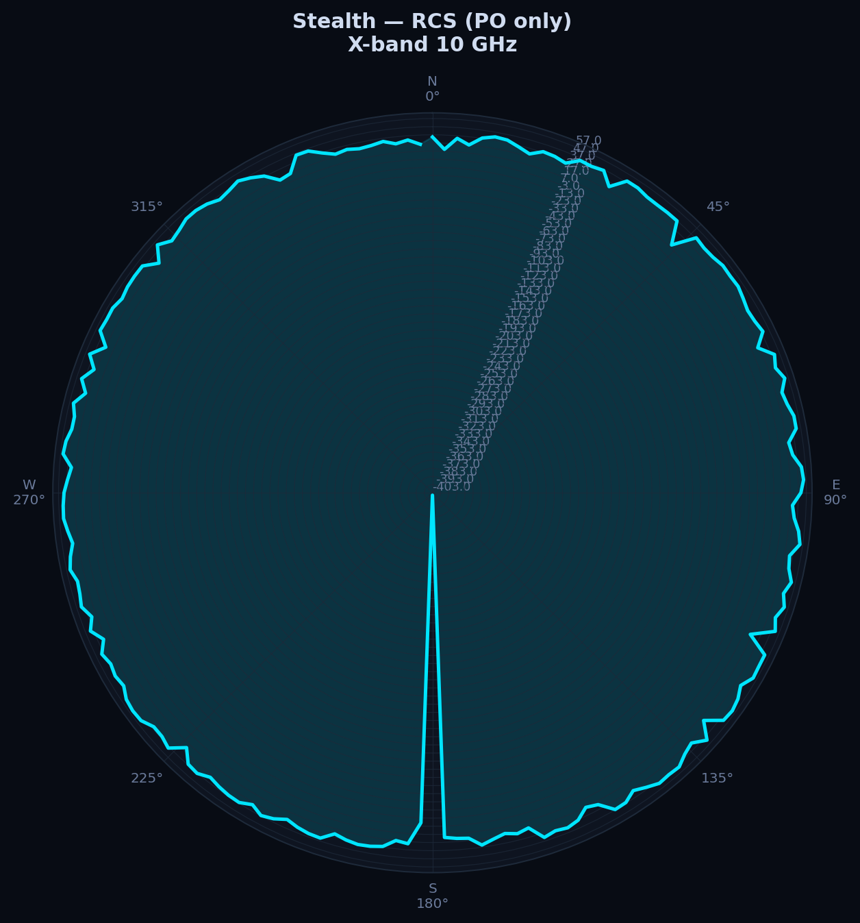
Limitation. PO-only computation underestimates RCS: it misses edge and multi-bounce contributions present in real geometries, and it has no concept of a shadow boundary's diffracted field (it just switches a facet fully on or fully off at the illumination boundary, which is physically discontinuous). Every subsequent layer below corrects a specific, named blind spot of PO.
3 Physical Theory of Diffraction (PTD), Edge Diffraction
Why it is needed. PO's tangent-plane approximation is only valid deep inside a flat facet; right at an edge, a wingtip, a trailing edge, the rim of an engine inlet, the surface is discontinuous and PO's prediction is not just imprecise, it is formally wrong (it predicts a field discontinuity across the shadow boundary that cannot physically exist, since Maxwell's equations forbid an infinitely sharp field transition). Ufimtsev's Physical Theory of Diffraction fixes this by adding a correction "fringe wave" localized to the edge itself, so the combined PO+PTD field is continuous everywhere, matching what a full-wave solution shows.
How it is computed. Ufimtsev's fringe-wave diffraction coefficient depends on the wedge's interior angle
via a parameter
Diffraction lobes from a finite edge of length
Where it matters for shaping. This is exactly why stealth aircraft leading and trailing edges are all swept to a small number of common angles ("edge alignment"), every edge's diffraction lobe then points in the same handful of directions, so there are only a few narrow "glint" aspects to defend against instead of edge energy smeared continuously across all azimuths.
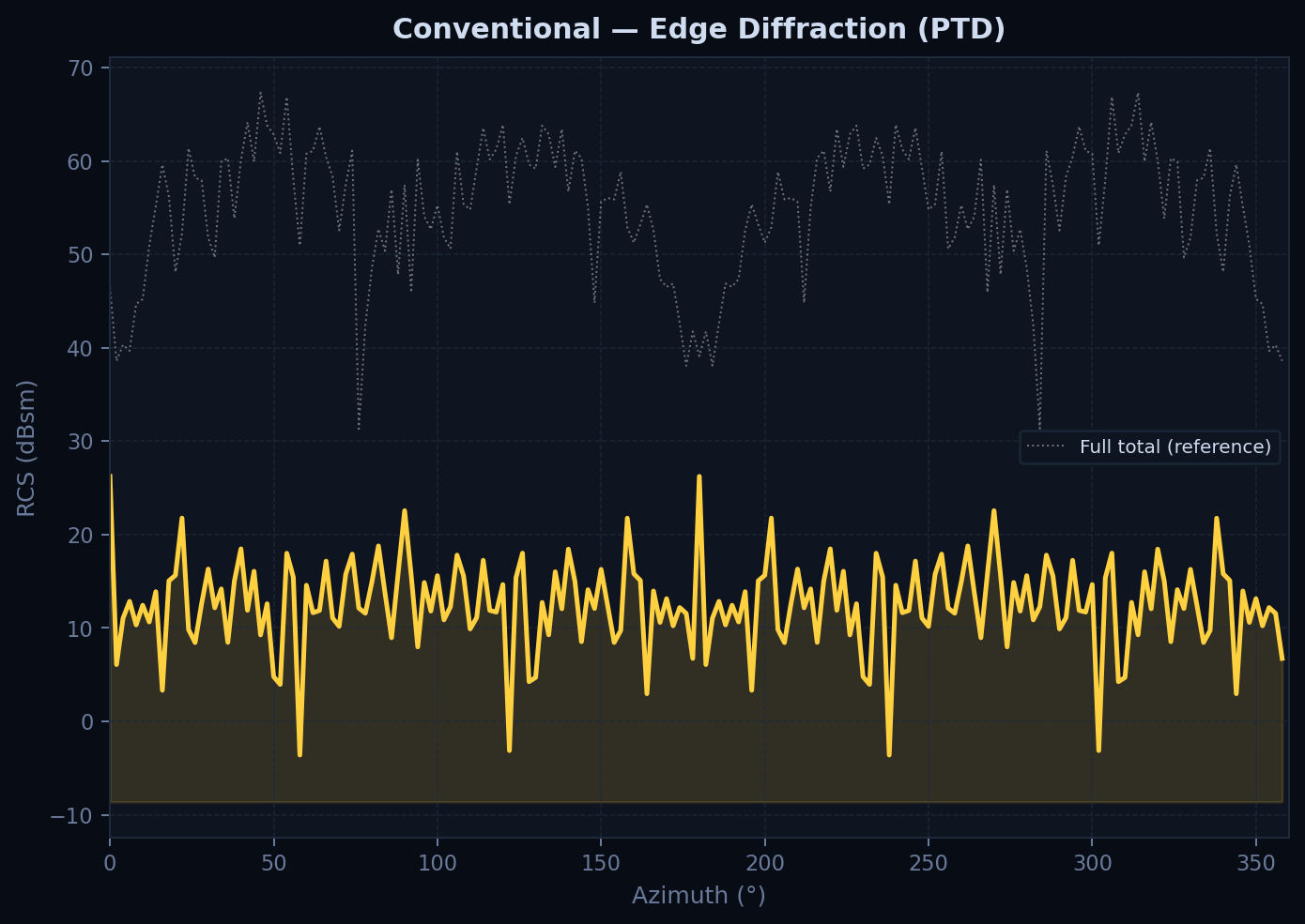
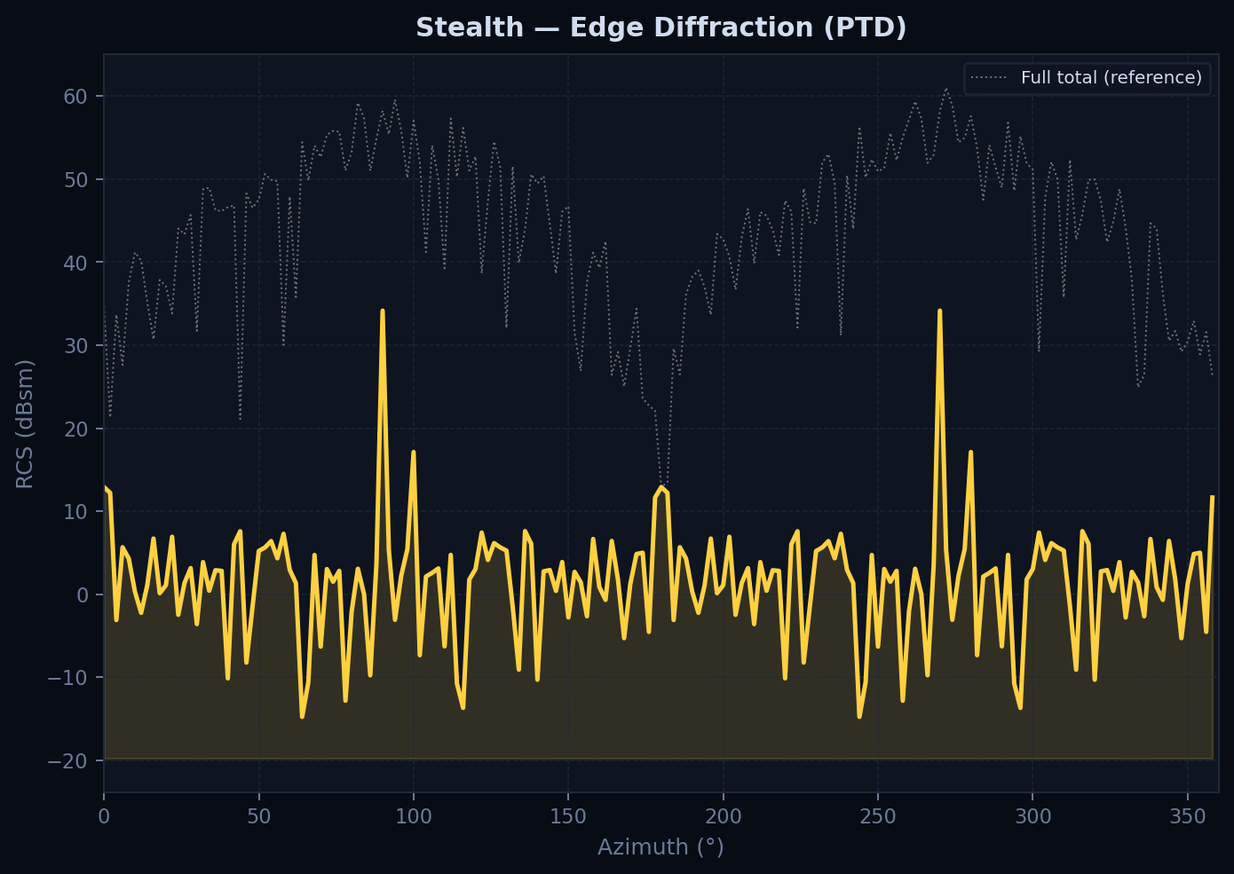
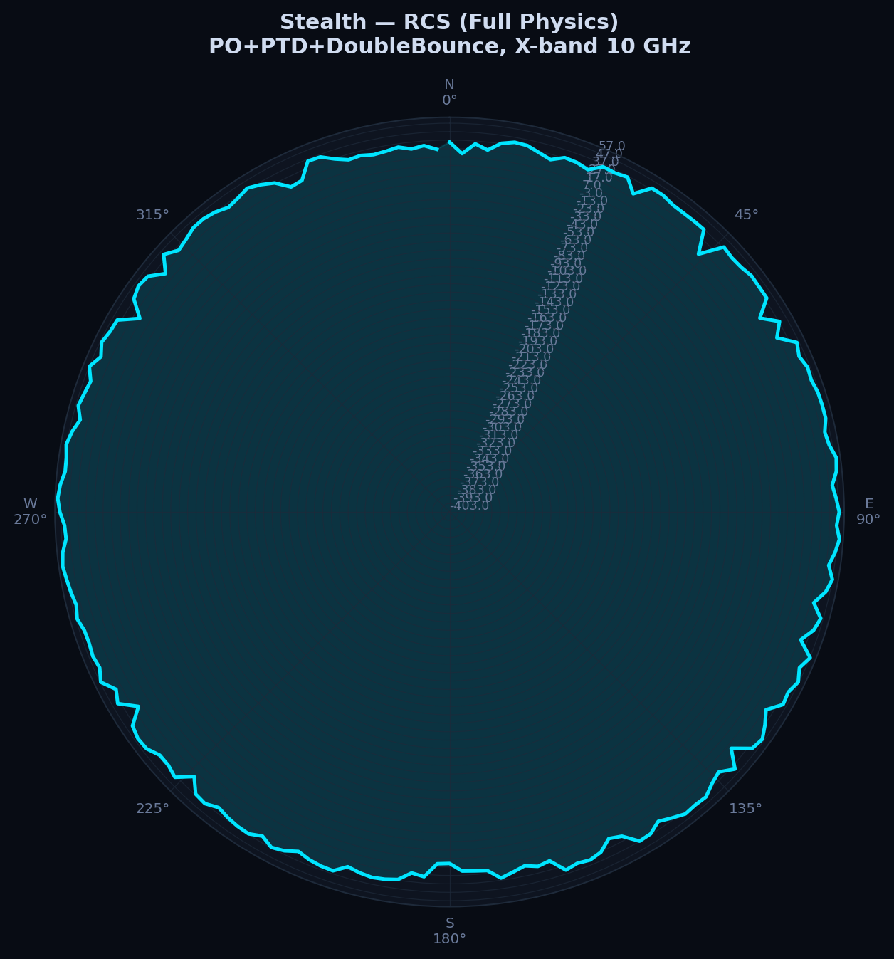
Adding PTD raises the mean RCS by capturing edge diffraction from geometric discontinuities that PO alone is blind to, visible as the elevated diffuse floor in every azimuth sweep on the Scattering Mechanisms tab.
4 Double-Bounce, Corner Reflector
What it is and why it is dangerous. Two flat facets meeting at close to a right angle form a dihedral
corner reflector, the same geometric principle used deliberately in navigation radar reflectors on small
boats (a cheap, lightweight way to make a fibreglass boat visible to ship radar) and in truck-mounted
calibration
targets. On an aircraft, a wing-fuselage junction or a fin-fuselage junction is an accidental version of
the
same thing: a ray hits the first facet, reflects onto the second facet, and reflects a second time
straight back along its incoming path, retroreflection, the same effect that makes a bicycle
reflector or road sign so bright when lit head-on by car headlights. A facet pair
where
5 Triple-Bounce, Trihedral Corner Reflector
What it is. Extending the ray trace one more reflection captures trihedral corners, three mutually near-perpendicular facets meeting at a point, exactly the geometry of a surveyor's or marine trihedral corner reflector (three metal or mesh panels folded like the inside corner of a cube), which is deliberately used as a radar calibration target precisely because it is such an efficient, wide-angle retroreflector. On an aircraft this three-way geometry shows up accidentally at a wing–fuselage–tail junction where three surfaces happen to meet at close to mutually perpendicular angles.
Why it returns even more energy than a dihedral. A trihedral reflects the incoming ray back along its
exact incoming path over a much wider solid angle of incidence than a dihedral does (a dihedral only
retroreflects
within the plane perpendicular to its fold line; a trihedral retroreflects over a genuine 3-D cone of angles),
and
its peak RCS scales with the fourth power of its characteristic edge length
Textbook-consistent finding: trihedral (triple-bounce) returns exceed dihedral
(double-bounce)
returns at their respective peak angles,
6 Bistatic Generalisation
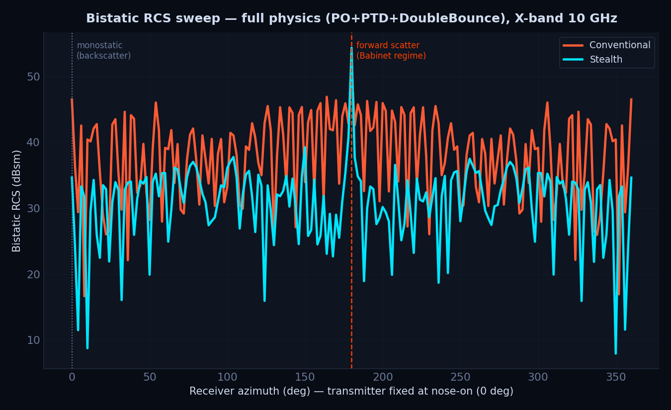
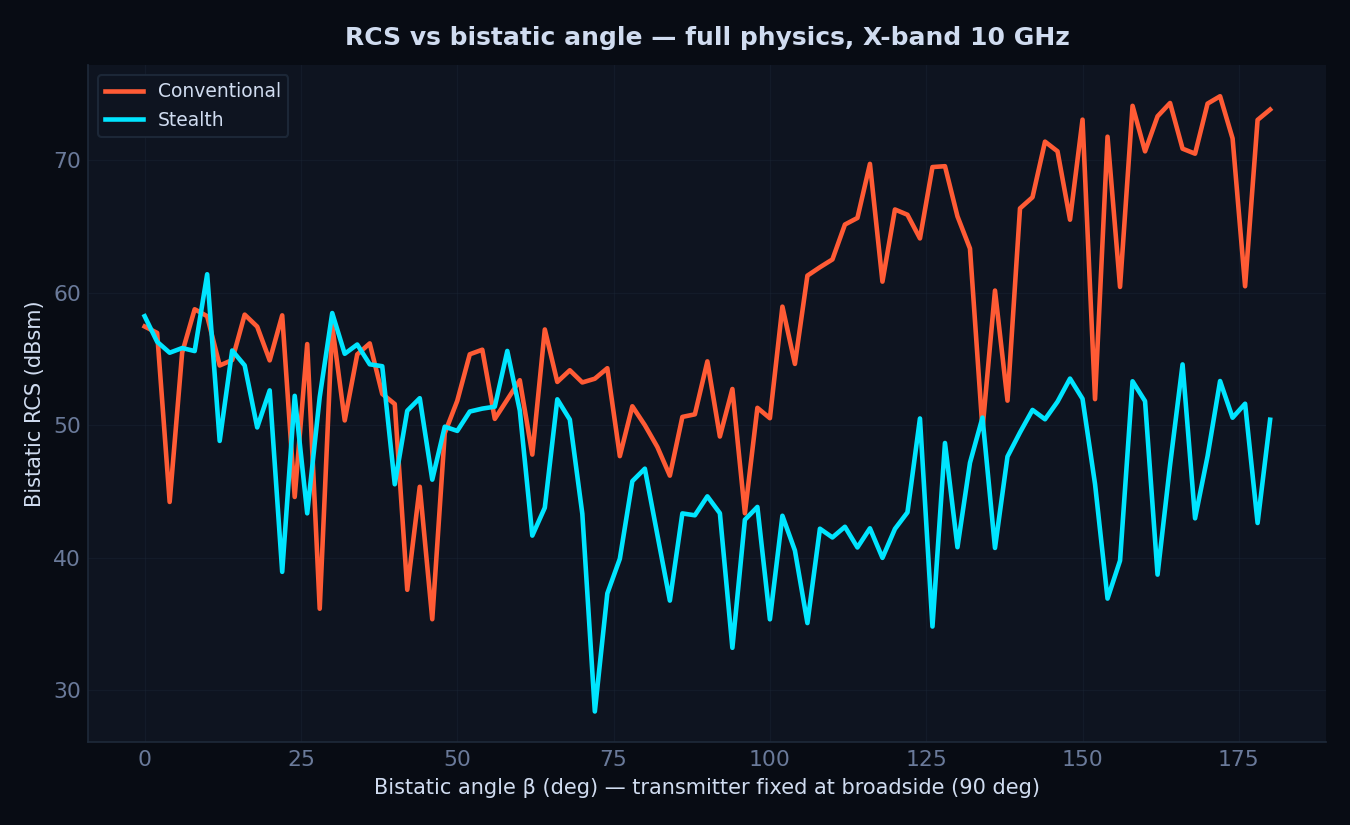
What "bistatic" means and why it is a separate case at all. Every equation above assumes the transmitter and receiver are co-located (monostatic radar, the ordinary case, one antenna doing both jobs). A bistatic radar instead has a physically separate transmitter and receiver, sometimes hundreds of kilometres apart. This matters for stealth because shaping a target to defeat monostatic detection (redirecting energy away from the transmitter) does not automatically defeat a receiver sitting somewhere else entirely, energy redirected away from one direction has to go somewhere, and a bistatic receiver can be waiting exactly there.
Where this is used in the real world. "Passive bistatic radar" or "passive coherent location" systems deliberately exploit this: they use existing FM radio or digital TV broadcast towers as the illuminator and a separate, silent (hence undetectable) receiver to pick up the forward-scattered or bistatically-scattered energy , a technique specifically discussed as a potential counter-stealth approach in open literature, because stealth shaping is optimized primarily for the monostatic backscatter case.
How the model generalises. All mechanisms above generalise to separate transmitter/receiver directions via the incidence–scatter bisector, physically, a facet reflects specularly relative to the bisector of the incoming and outgoing ray directions, exactly like a mirror, so the obliquity and phase terms are evaluated against that bisector instead of a single direction:
At
7 Polarimetric RCS
What it is and why a single RCS number is not the whole story. Radar antennas transmit a specific polarization (horizontal H or vertical V) and can also receive on either polarization. A real target can shift some of the reflected energy from the transmitted polarization into the orthogonal one, "depolarization" or "cross-pol return", and how much it does so is itself a distinguishing physical signature, not noise. A full 2×2 complex scattering matrix relates incident to scattered field in a fixed global (H,V) basis:
How depolarization physically arises. Each PEC facet reflects with the textbook TE/TM dichotomy
(
8 RAM, Salisbury Screen & Dallenbach Layer
What RAM is and why shaping alone is not always enough. Radar-Absorbent Material is a coating or layer
applied to a surface specifically to convert incident RF energy into heat (dielectric or resistive loss) instead
of reflecting it. Shaping cannot help everywhere, some surfaces (a necessarily-flat weapons-bay door, an
engine inlet lip) cannot be angled away from every possible threat direction without breaking some other
requirement, and RAM is the tool that reduces the return from exactly those surfaces without changing their
shape.
Both classical designs modelled here are transmission-line reflection problems: a resistive/lossy layer over a
PEC backplane (representing the aircraft's underlying metal structure), characterised by an input impedance
Salisbury screen, a single resistive sheet (
Dallenbach layer, a single lossy dielectric slab (complex
Loss is distributed through the slab volume rather than concentrated at one sheet: broader but shallower absorption than Salisbury, i.e. it trades peak absorption depth for a wider useful frequency band, which is generally the more practical trade-off for an aircraft that must stay stealthy across an entire radar band, not just one calibration frequency.
9 Surface Impedance Boundary Condition (SIBC)
Every mechanism above assumes a Perfect Electric Conductor (
Why it's required. Modern airframes increasingly use CFRP composites (conductivity ~1000× lower than aluminum) instead of aluminum skins, a PEC-only model cannot distinguish them. SIBC plugs a real, measurable material property directly into every existing solver via the same interface used for Salisbury/ Dallenbach RAM, with zero physics-layer rewrite.
10 Geometry Optimization
Why automate the search at all. Everything up to this point treats the stealth aircraft's shape as fixed, a human designer picked the sweep angle, the tail cant, and the nose length by hand, informed by the design principles in §3–5 above. But those design principles only say the direction to move a parameter (sweep more, cant more); they do not say the specific optimal value, and RCS depends on all three parameters simultaneously through a landscape that is far too complex to search by hand. This section asks: if we let the computer search that parameter space automatically, can it beat the hand-tuned baseline, and by how much?
How the problem is set up. Stealth geometry is parametrized by wing leading-edge sweep angle
Why differential evolution, not gradient descent. Solved with
Where this mirrors real aircraft design practice. Modern aircraft design increasingly uses exactly this kind of multi-disciplinary automated optimization (MDO), letting an algorithm search a shape's free parameters against a stated objective (RCS, drag, structural weight) rather than relying purely on a human designer's iteration-by-hand, though a real MDO loop runs alongside aerodynamic and structural constraints this teaching-scale version deliberately leaves out to keep the search tractable and its result explainable.
11 Wideband Impulse Response
Why a single frequency is not enough. A single number cannot tell you where along the aircraft the energy is coming from, the nose, a wing leading edge, and the tail can all contribute to the same one-number total, indistinguishably. Real radars that need that spatial information (range profiling, target recognition) do not transmit one frequency; they step or sweep across a band and combine the results. This section reproduces exactly that processing chain.
How it works. Instead of a single-frequency RCS number, sweep the same coherent complex amplitude across a frequency band and inverse-Fourier-transform it into a time-domain range profile, the standard stepped-frequency radar processing chain used to resolve individual scattering centres along the target's line of sight. Physically: each frequency in the sweep is a different "comb tooth"; Fourier theory guarantees that combining many closely-spaced frequency-domain samples and inverse-transforming them synthesizes a short time-domain pulse, exactly as if a single very-short, very-wideband pulse had been transmitted and its echo recorded directly , without ever needing hardware capable of generating that short a pulse.
Geometry & Meshing
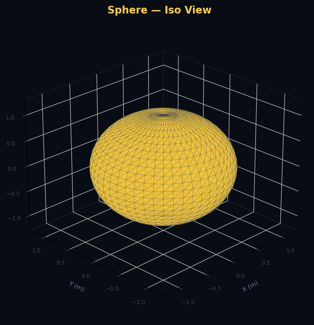
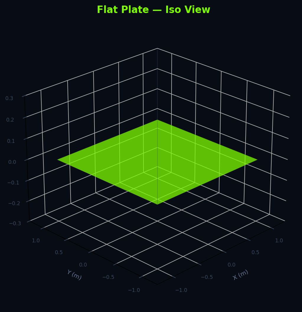
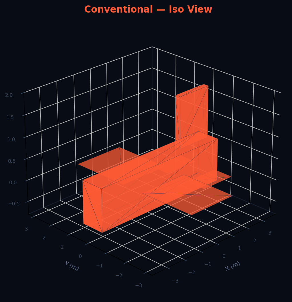
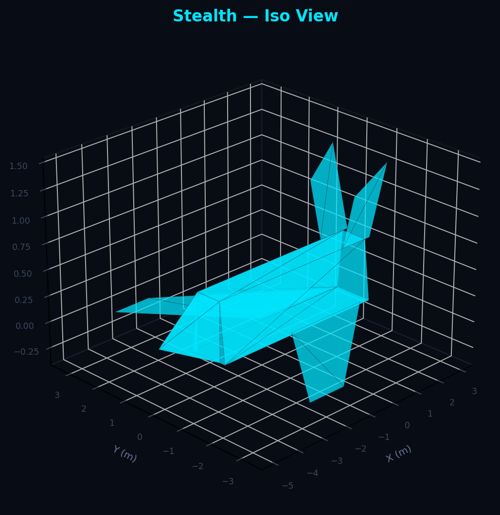
Six triangulated-mesh PEC geometries, all built from first-principles facet primitives
(
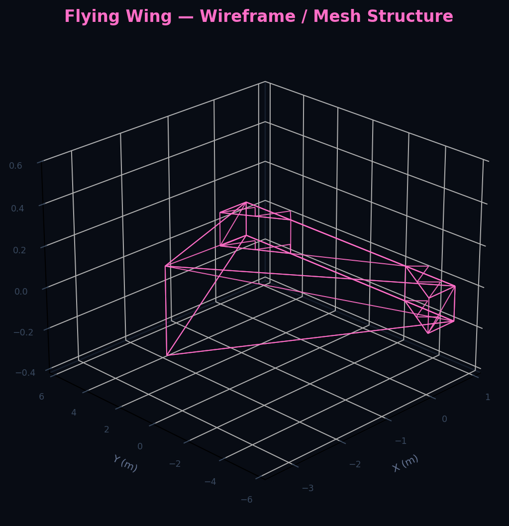
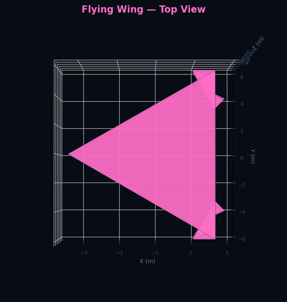
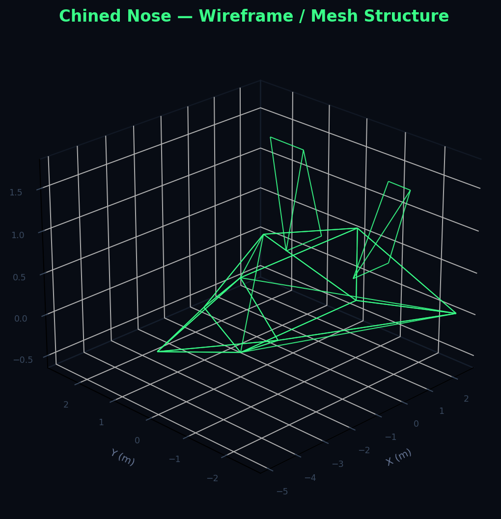
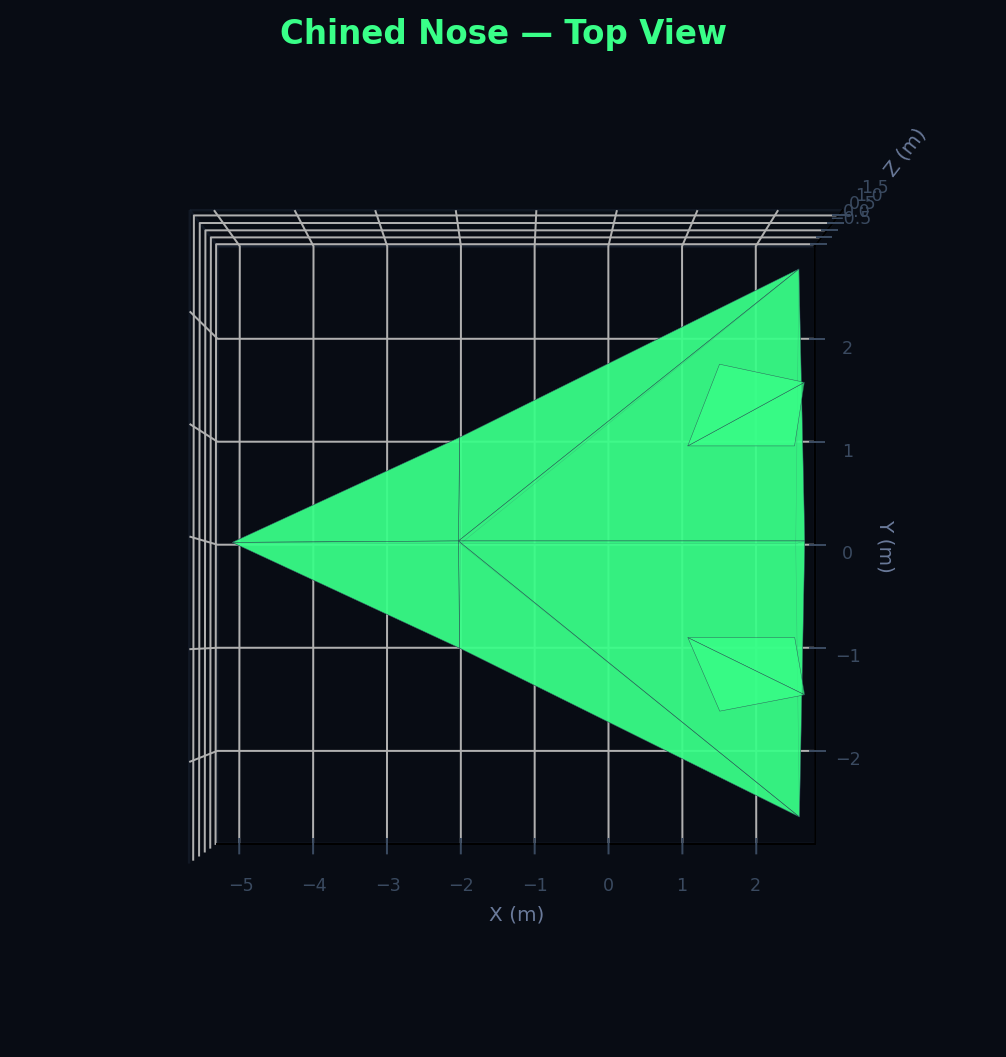
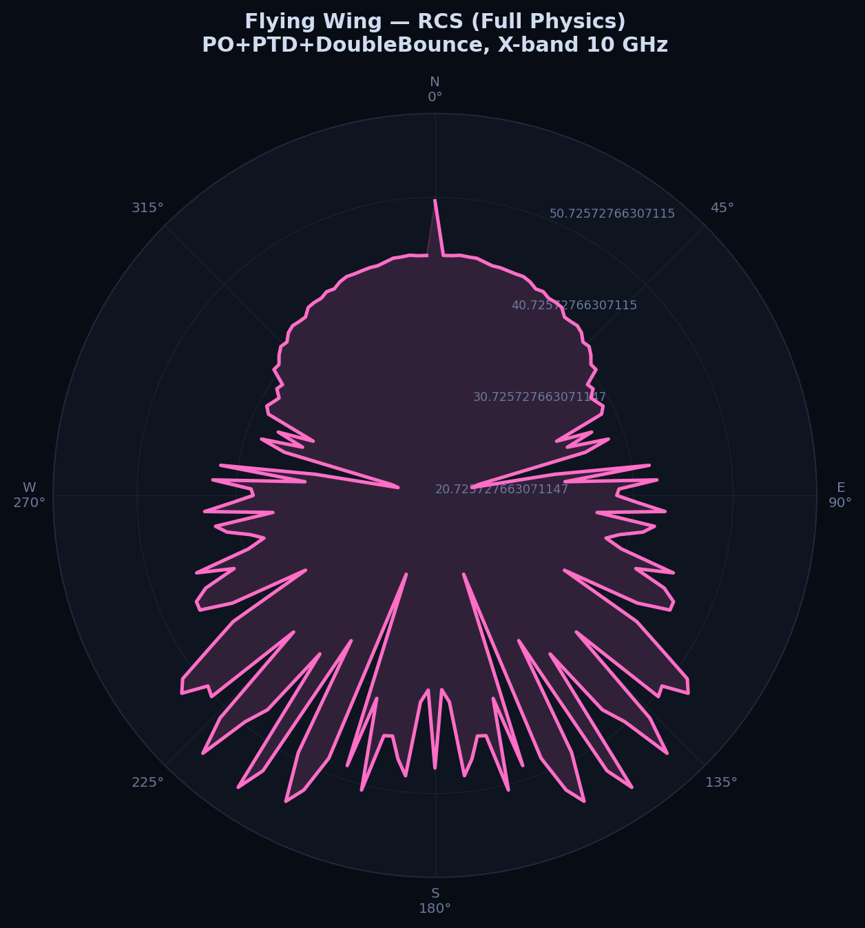
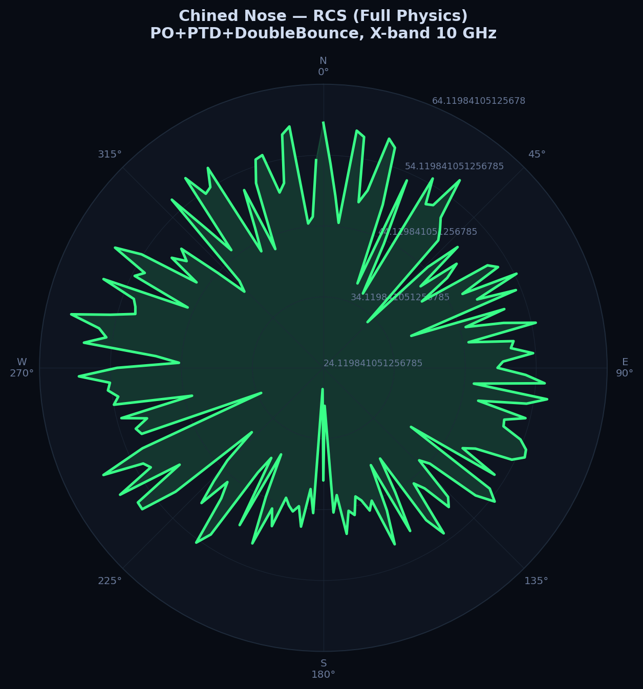
Why six shapes and not just "conventional vs stealth"? Each of the other four isolates one specific electromagnetic idea so its effect can be seen in isolation before looking at the two full aircraft: the sphere is the one shape with an exact closed-form answer (used purely to validate the solver, see §4 below); the flat plate is the simplest possible specular reflector, used as a textbook-formula sanity check; the flying wing demonstrates a shape with zero vertical surfaces at all (the most radical stealth shaping choice, used on the real B-2 Spirit); and the chined-nose shape demonstrates blending the fuselage directly into the wing leading edge (used on the real F-22/F-35 family) as an alternative to a separate, sharply-defined nose cone.
1 Target Geometries
| Geometry | Baseline facets | Notes |
|---|---|---|
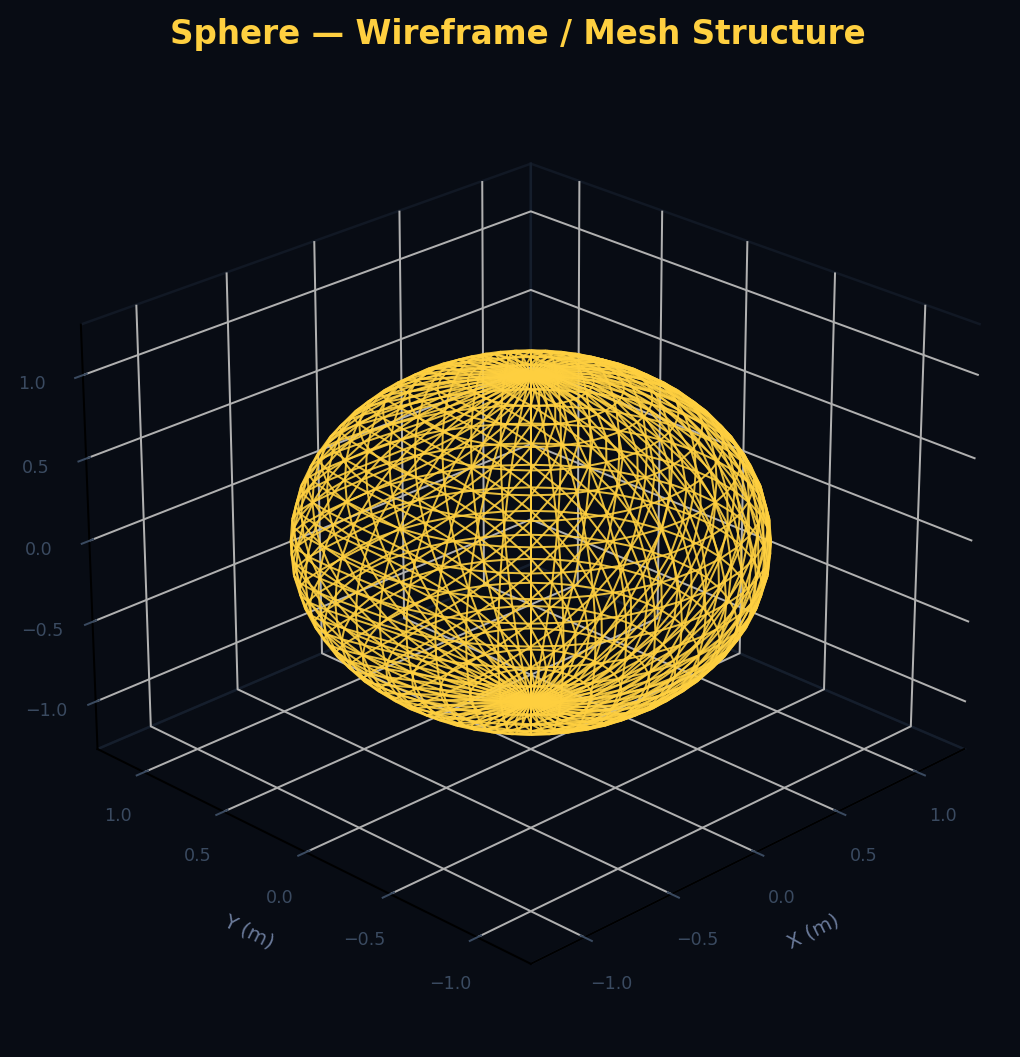
| Sphere (r=1 m) | 2304 | Mie-series validation baseline |
| Flat plate (2×2 m) | 2 | Textbook |
| Conventional aircraft | 34 | Flat fuselage, right-angle wing/fin dihedrals, flat nose-on intake |
| Stealth aircraft | 20 | Trapezoidal fuselage, pyramidal nose, 65° swept delta wings, 35°-canted V-tail |
| Flying wing | 28 | Zero vertical surfaces, sawtooth trailing edge |
| Chined nose | 18 | Diamond fuselage blended to wing LE, 28° twin tails |
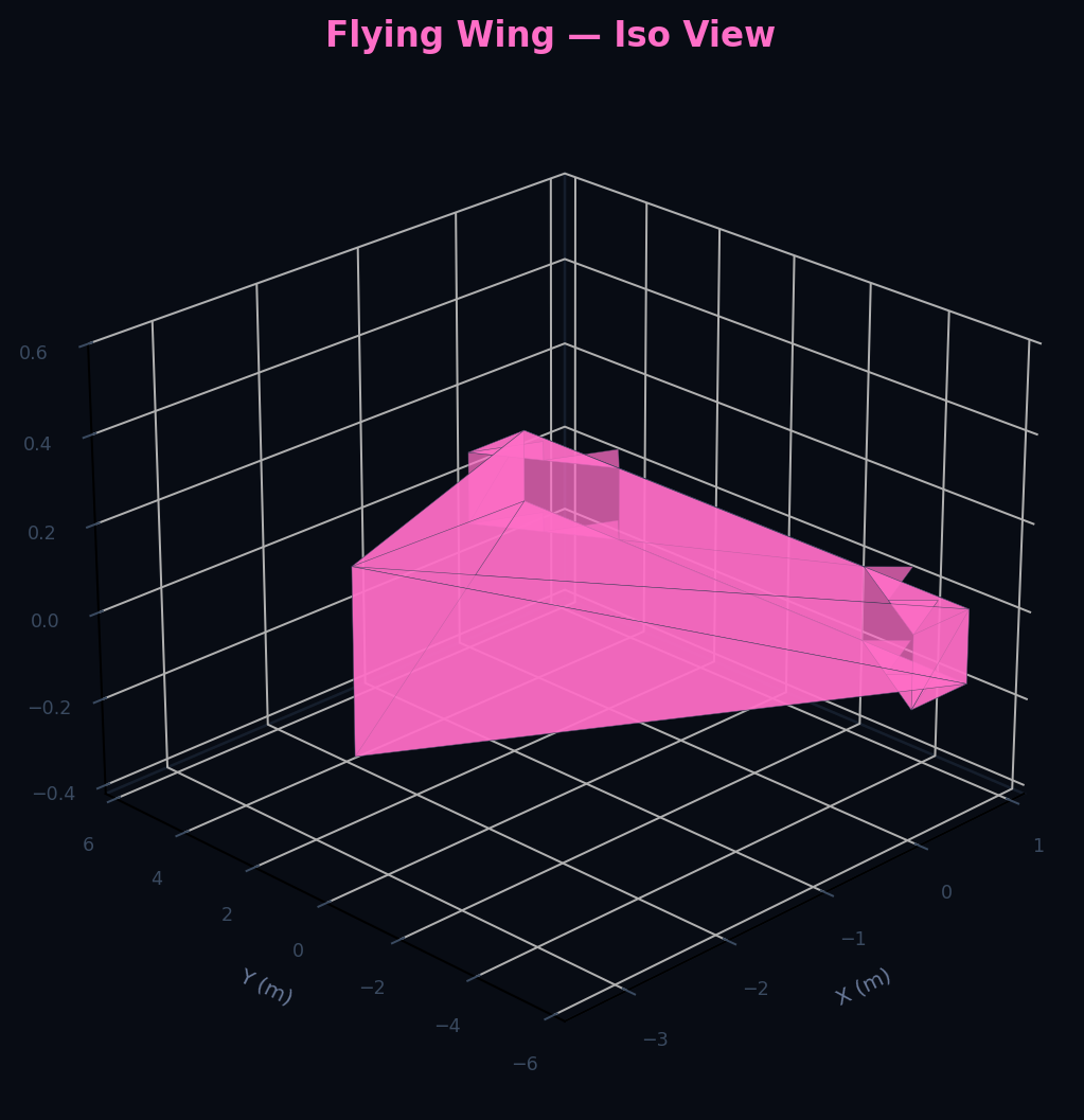
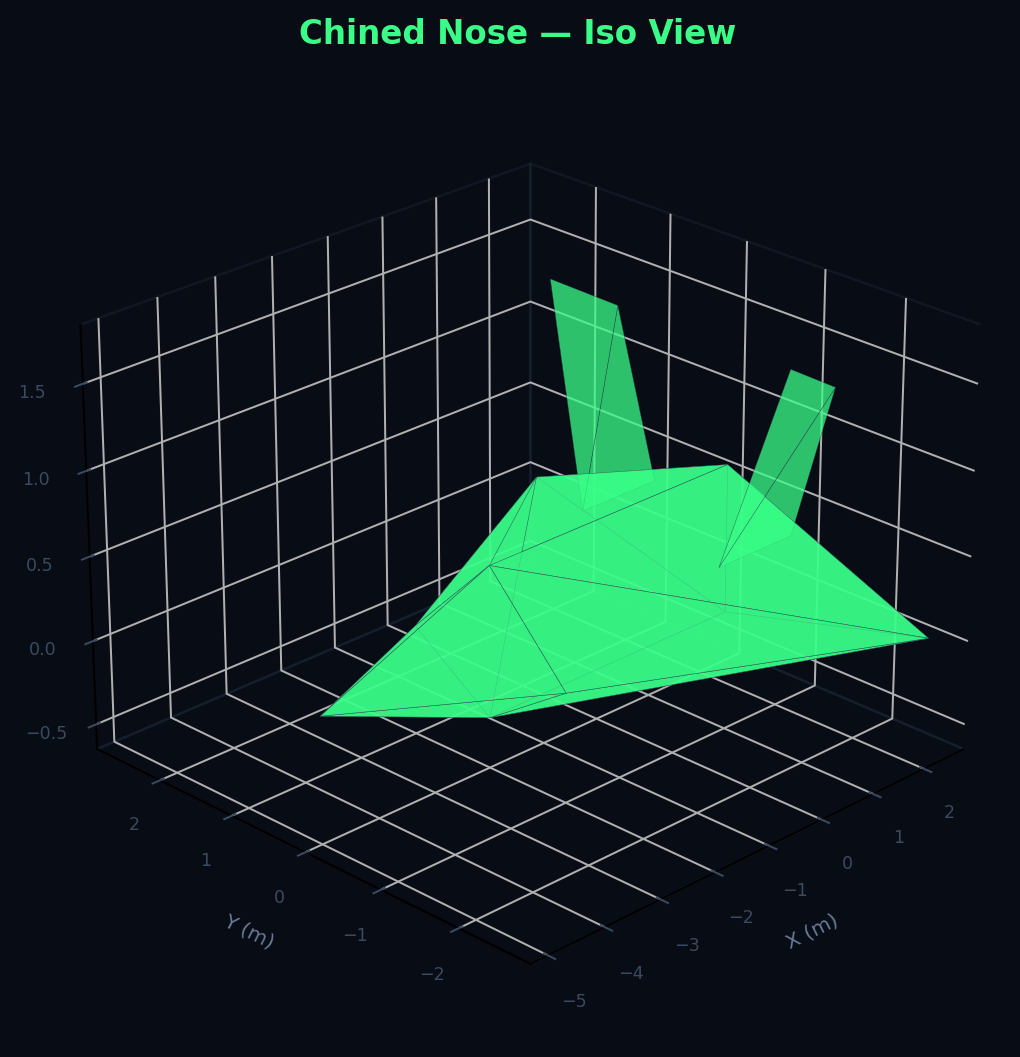
2 Multi-View Detail (Conventional vs Stealth)
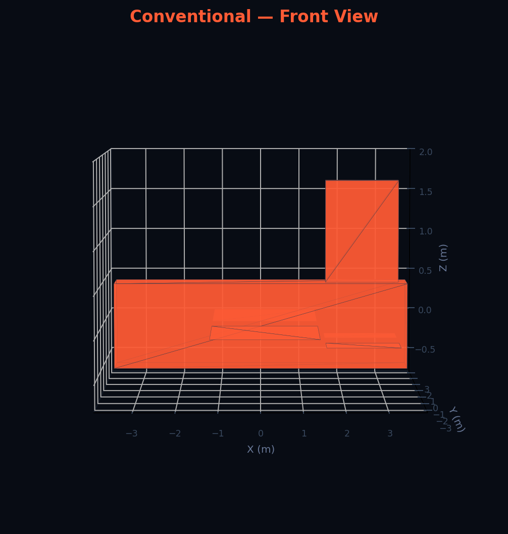
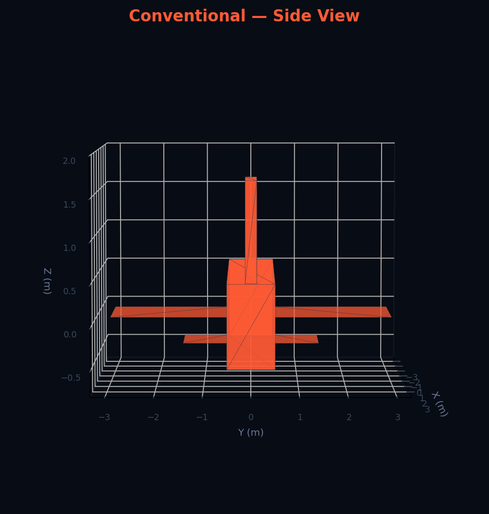
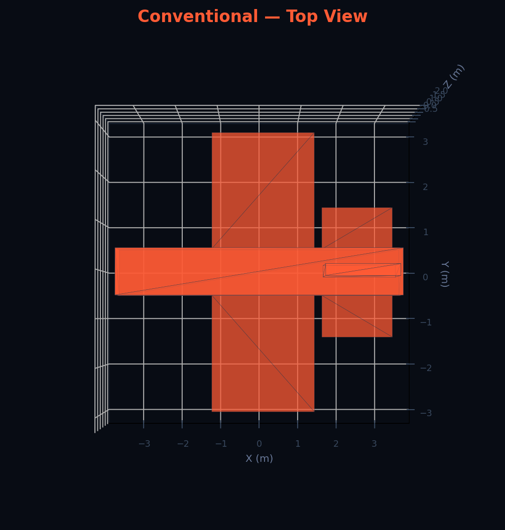
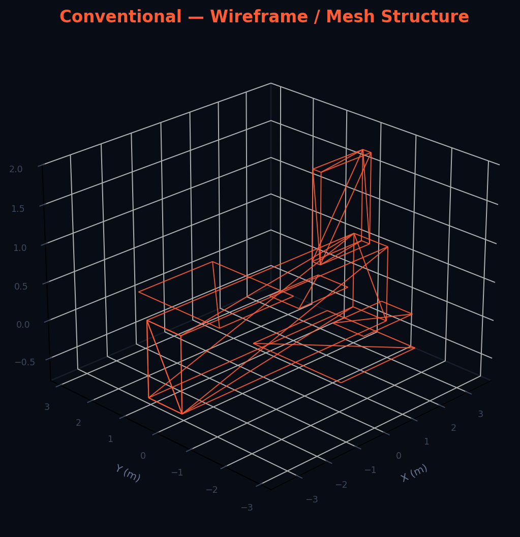
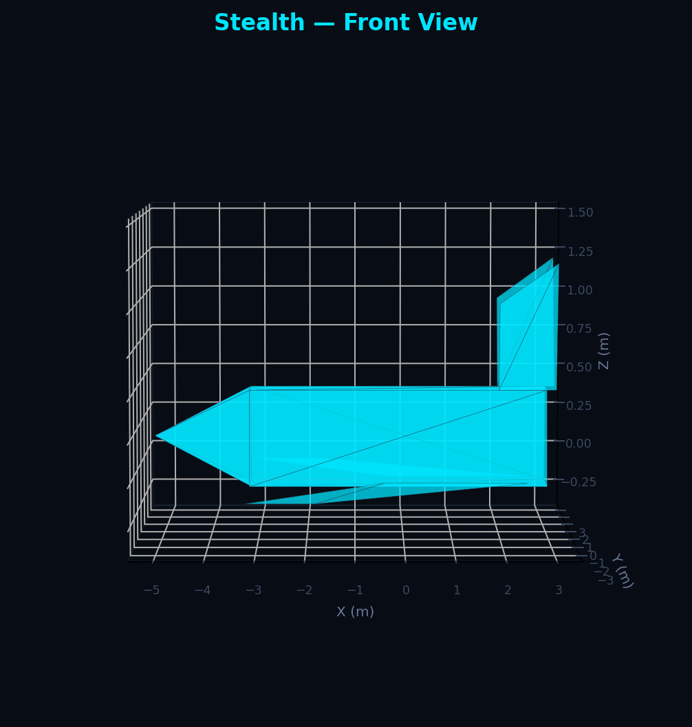
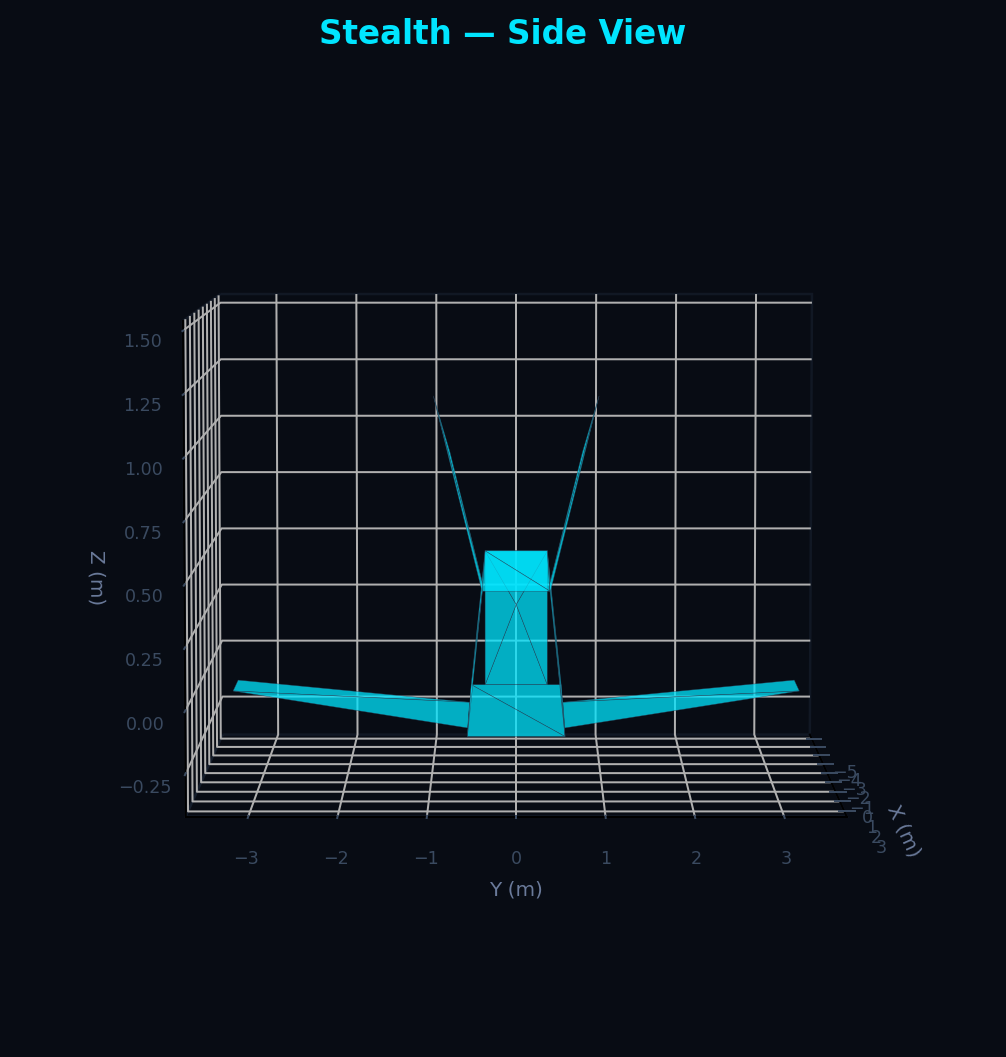
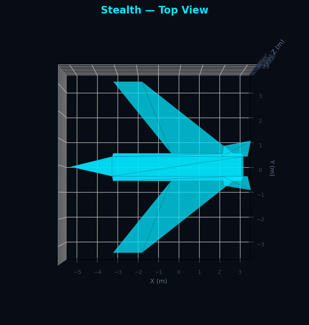
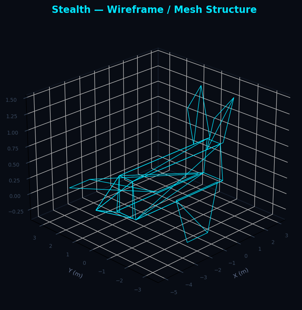
Flying wing & chined nose
3 Edge Classification
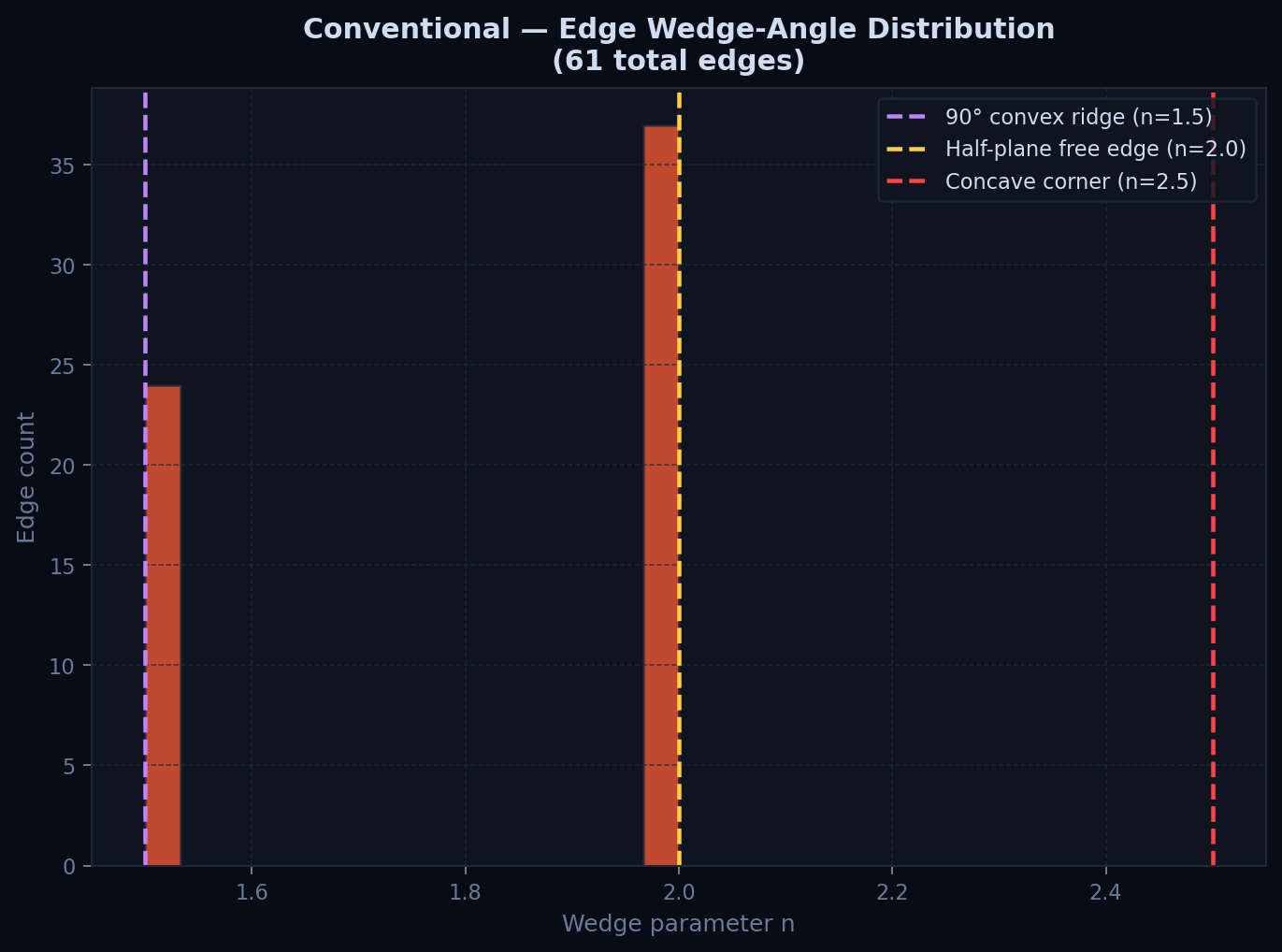
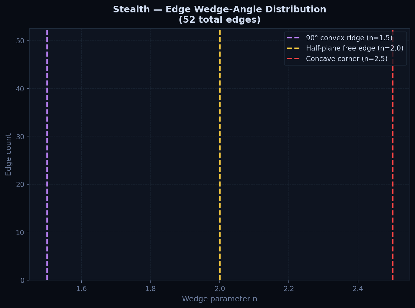
Why classify edges at all. Recall from the Governing Physics tab that PTD's diffraction strength depends
on the wedge parameter
| Geometry | Total edges | Internal edges | Boundary edges | Mean wedge n |
|---|---|---|---|---|
| Conventional aircraft | 61 | 41 | 20 | 1.8 |
| Stealth aircraft | 52 | 8 | 44 | 2.0 |
The conventional aircraft's 41 internal edges (many at
4 Mie Validation (Why Trust the Solver)
5 Mesh Convergence, Baseline (PO+PTD+DoubleBounce)
Why bother checking this. The report's headline numbers use deliberately coarse baseline meshes (18–34 facets) chosen to keep the O(n2) double-bounce and O(n3) triple-bounce solvers fast enough for interactive sweeps across hundreds of angles. That raises an obvious, fair question a reviewer should ask: is 20–34 facets actually enough, or are the headline numbers an artifact of too coarse a mesh? A mesh-convergence study is the standard numerical-methods answer to exactly that question, refine the mesh repeatedly and check whether the answer stops changing. If it does not stop changing, the original result cannot be trusted regardless of how physically reasonable it looks.
Does RCS stabilise as facet count grows and facet size shrinks well below
Why the curve suddenly jumps at two points instead of smoothly flattening. Look
closely and every convergence chart on this site has one or two sudden steps rather than a single smooth
settle, those steps sit exactly where the plot crosses from one solver tier to the next
(DoubleBounce→PTD around 8,704→34,816 facets, PTD→PO around 557,056→3,060,000 facets).
This is not numerical error and not the mesh failing to converge. Double-bounce and PTD are too
expensive to run at millions of facets (
Scattering Mechanism Breakdown
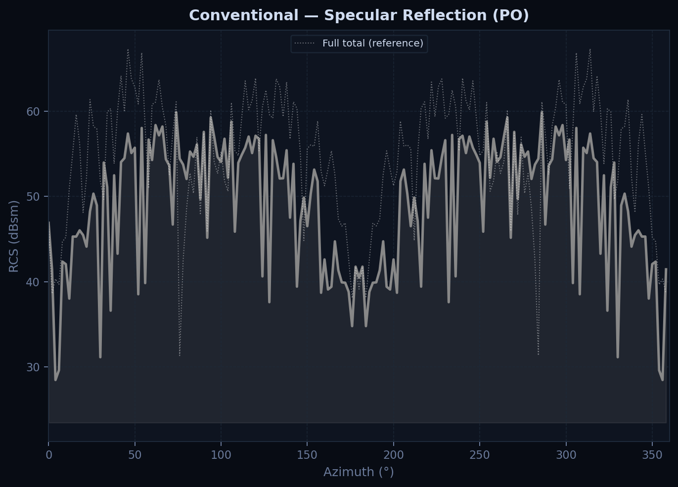
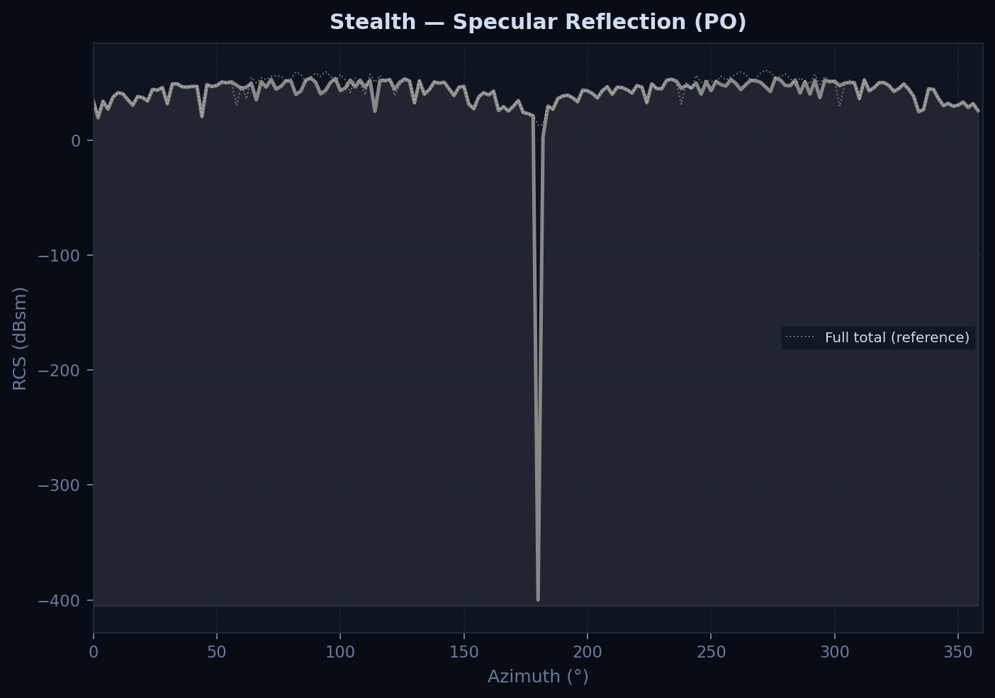
Isolating each physics layer (PO-only, PTD edge, double-bounce) on the same axes reveals which geometric feature drives which mechanism, the diagnostic result the problem statement explicitly demanded (Challenge 3, Overview §2). This is the tab that turns "the total RCS is X dBsm" into "the total RCS is X dBsm, and here specifically is what caused it and where on the airframe."
The method is simple: compute the same azimuth sweep three separate times, once with only the PO layer switched on, once with only PTD, once with only double-bounce, and plot each against the full-physics total as a faint reference line. Wherever a single-mechanism curve tracks close to the full-physics line, that mechanism is the dominant contributor at that angle; wherever it sits far below, something else (usually one of the other two layers) is doing most of the work there instead.
1 PO-Only (Specular)
2 PTD Edge Diffraction
3 Double-Bounce (Corner Reflector)
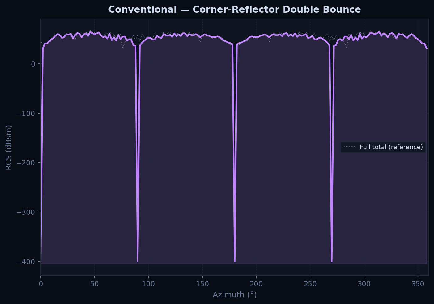
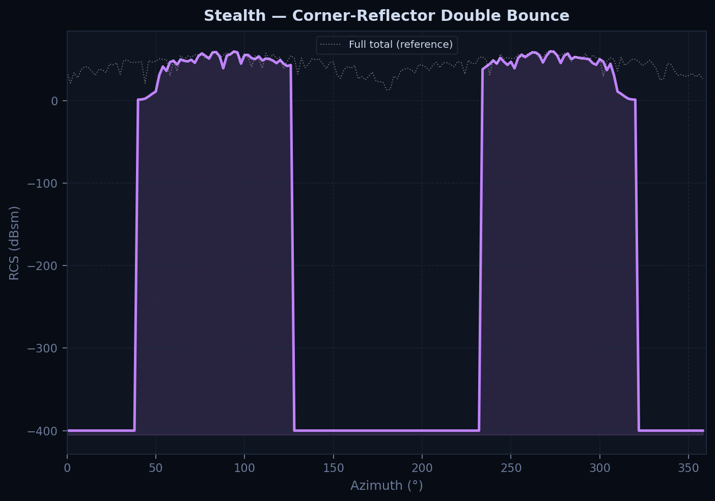
Double-bounce hotspot count. Conventional aircraft: 48 active retroreflecting facet pairs clustered at the fin–fuselage 90° dihedral. Stealth aircraft: ~22 pairs at roughly half peak amplitude with no dominant cluster, the 35°-canted V-tail eliminates the dominant corner reflector rather than merely weakening it.
4 RAM Physics Diagrams
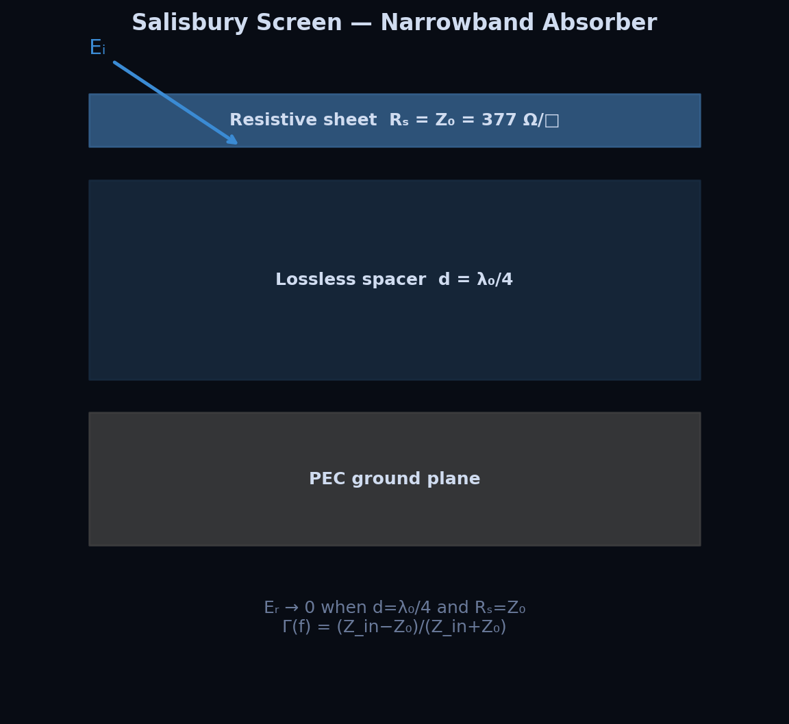
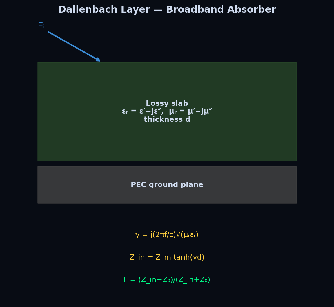
5 Design Principles Derived From the Breakdown
- Sweep leading edges. Shifts the diffraction peak by angle
\Lambda off nose-on, moving the return outside the frontal threat corridor for\Lambda>60^\circ . Evidence: stealth aircraft's ~65° swept delta wings with aligned trailing edges. - Cant vertical surfaces. A single design change simultaneously reduces specular return and eliminates the 90° fin–fuselage double-bounce corner. Evidence: stealth V-tails canted 35° outward.
- Combine shaping with RAM. Shaping redirects scattered energy away from the threat sector; RAM reduces the amplitude of remaining returns, Salisbury screens give deep narrowband absorption, Dallenbach layers give broader shallower absorption.
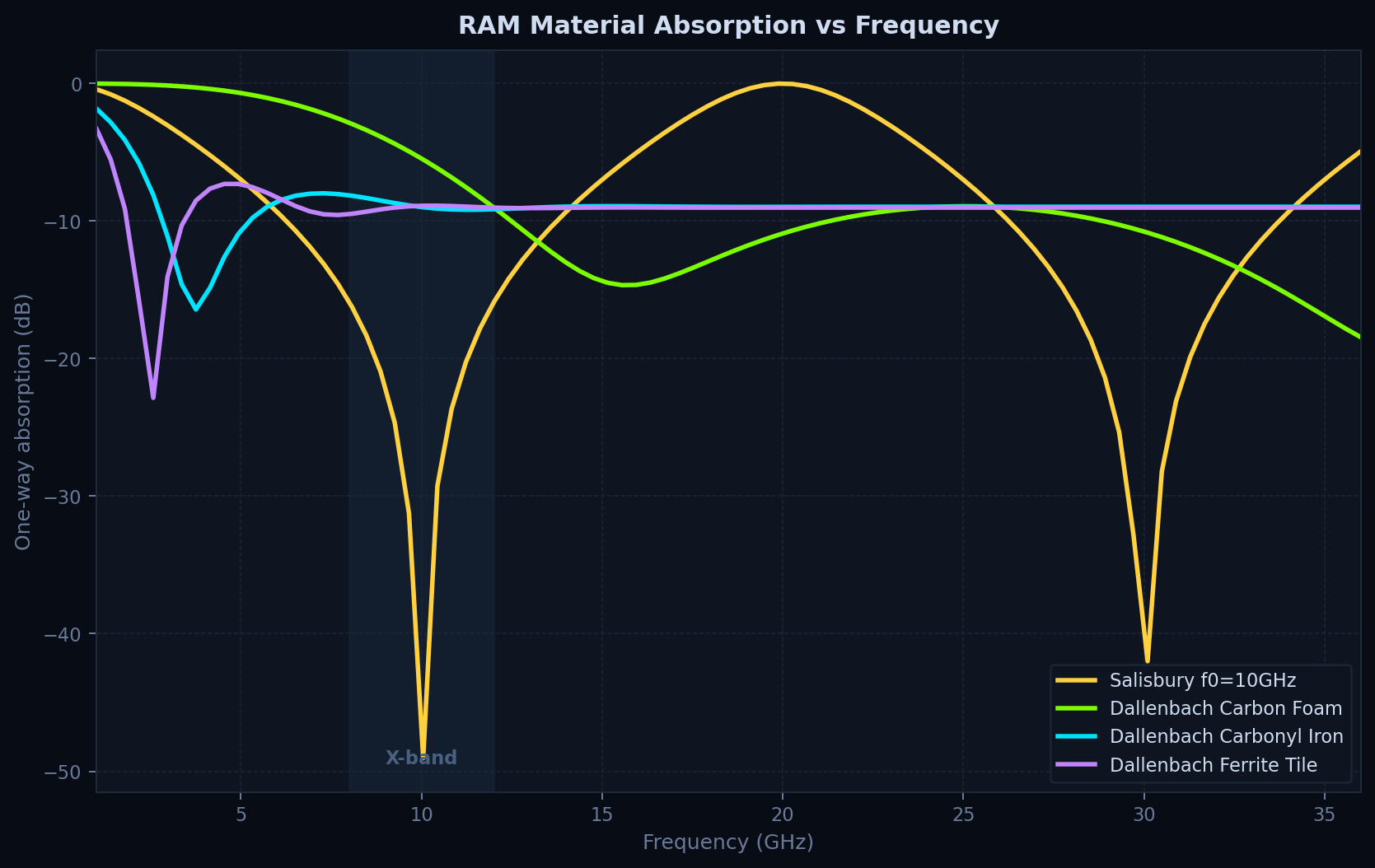
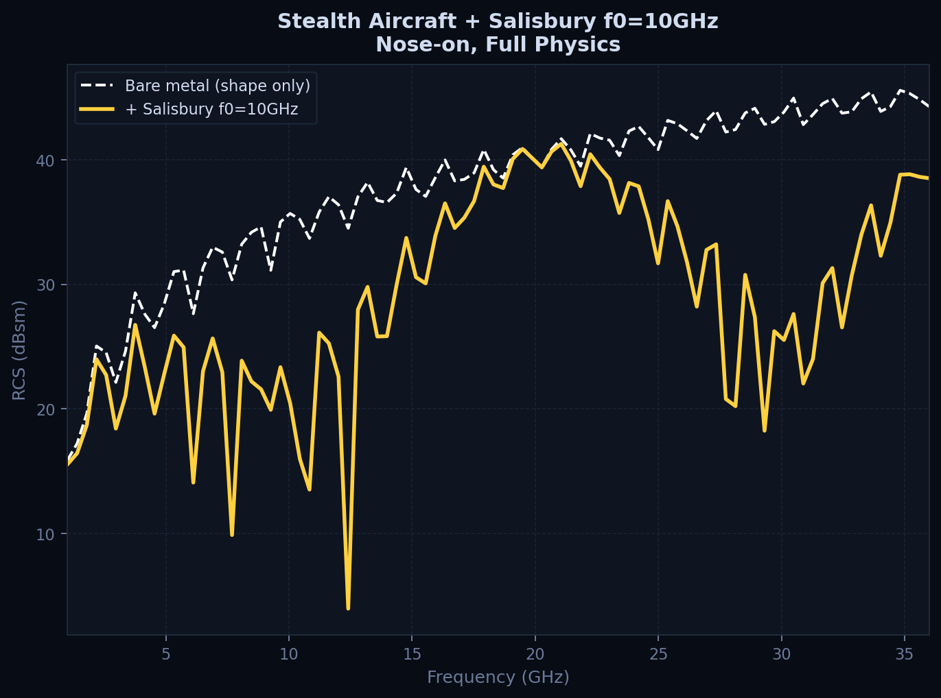
Bistatic & Polarimetric RCS
Extending every solver (PO, PTD, double-bounce, triple-bounce) to independent transmit/receive directions and to the full 2×2 polarimetric scattering matrix, both generalisations verified bit-for-bit to reduce to their monostatic/scalar forms when tx=rx. Formulation and real-world motivation for both extensions is in Governing Physics §6–7; this tab is the results.
1 Bistatic Sweep
2 Polarimetric Signature
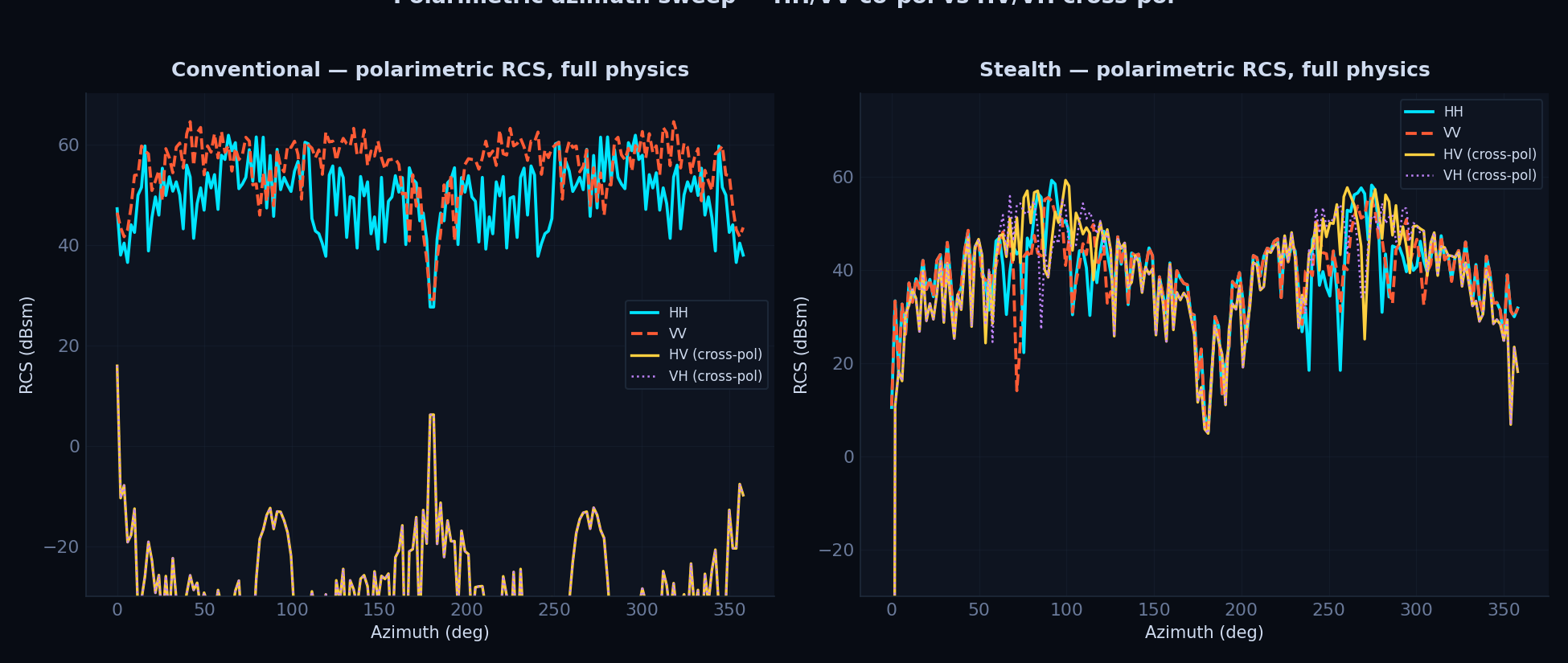
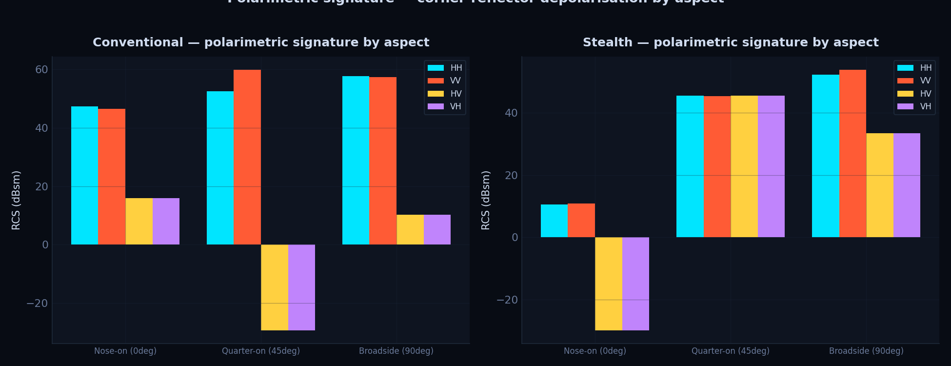
Flat plate at normal incidence: HH=VV, HV<−60 dB below co-pol (numerically zero, no plane of incidence, no depolarisation). Corner reflector at 45°: full-physics HV exceeds PO-only HV by >3 dB, the double-bounce cascaded-Jones term is what produces real cross-pol.
3 Mesh Convergence, Bistatic RCS
Same tiered solver strategy; bistatic pair az_tx=0°/el_tx=0°, az_rx=30°/el_rx=10°.
4 Mesh Convergence, Polarimetric (HH / HV)
Multi-Bounce: Double-Bounce vs Triple-Bounce
Extending the double-bounce ray trace one more reflection captures trihedral corners (wing–fuselage–tail three-way junctions), a real conventional-aircraft mechanism absent from the two-bounce model. Why trihedrals matter and how the peak-RCS formula is derived is covered in Governing Physics §5; this tab is the numerical evidence, including the honest admission that the triple-bounce mesh-convergence study below did not fully converge given practical compute limits.
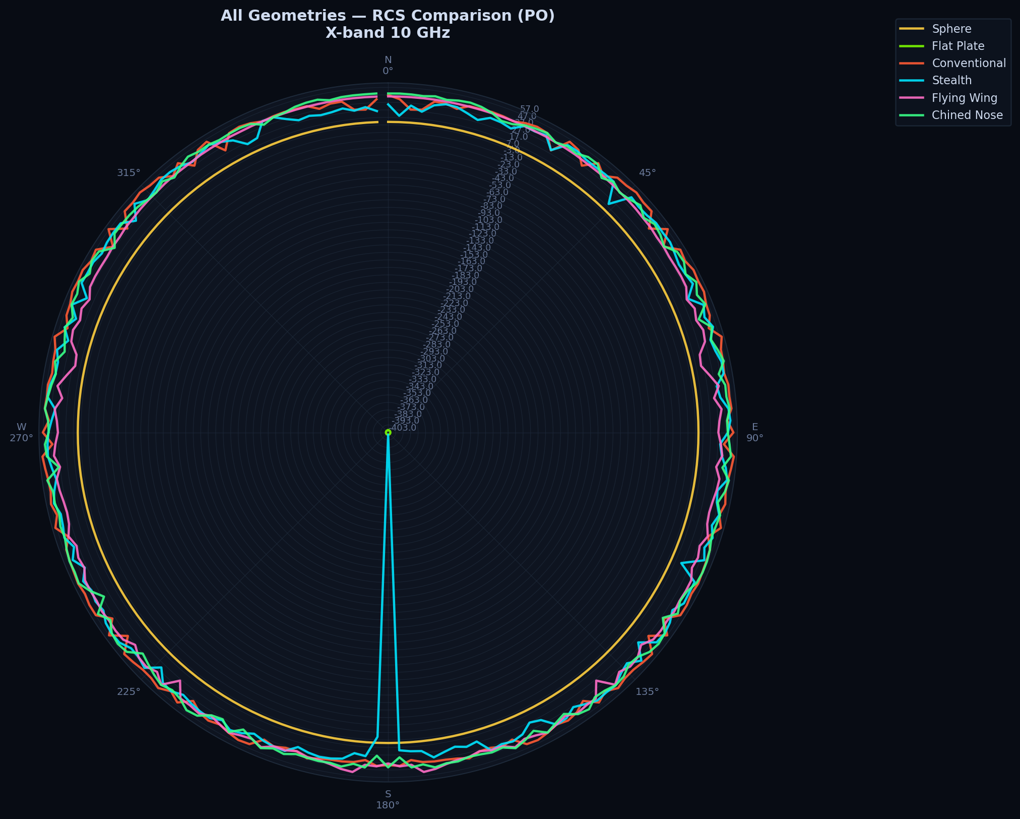
1 Corner-Reflector Comparison (Full Azimuth)
2 Mesh Convergence, Triple-Bounce (Scalar)
Peak trihedral angles located by coarse sphere sweep: Conventional az=85°/el=60°, Stealth az=340°/el=60°. Dashed = double-bounce reference at the same angle for scale.
3 Mesh Convergence, Triple-Bounce Polarimetric
4 Physical Interpretation
Peak trihedral RCS exceeds peak dihedral RCS for both geometries at their respective
optimum
angles, textbook-consistent (
RAM & Surface Impedance Boundary Condition
PEC vs finite-conductivity real aerospace skins, X-band and swept frequency, using the Leontovich SIBC (see Governing Physics §9) plugged into every existing solver via the same interface as Salisbury/ Dallenbach RAM.
Every plot before this tab assumed a Perfect Electric Conductor, a mathematical idealisation with infinite conductivity that reflects 100% of incident energy. Real airframe skins are not PEC: aluminum, titanium, and especially modern carbon-fibre composite (CFRP) skins are finite conductors. This tab asks the natural next question a materials-aware reviewer asks: does that idealisation actually matter, or is PEC a safe enough approximation for RCS work? The answer, worked out quantitatively below rather than assumed, turns out to be aspect- and frequency-dependent, PEC is an excellent approximation at X-band for every material tested, but the approximation visibly degrades as frequency rises.
1 Real Material Conductivities Used
| Material | Conductivity σ (S/m) | Typical use |
|---|---|---|
| Aluminum 2024-T3 | 1.74×10⁷ | Conventional airframe skin |
| Stainless steel 304 | 1.45×10⁶ | Fasteners / ducting |
| Titanium Ti-6Al-4V | 5.80×10⁵ | Structural / hot-section |
| CFRP composite | 3.0×10⁴ | Modern composite skin (worst conductor here) |
Approximate, room-temperature, commonly-cited engineering reference values.
2 PEC vs Real Materials, Azimuth Sweep, X-band
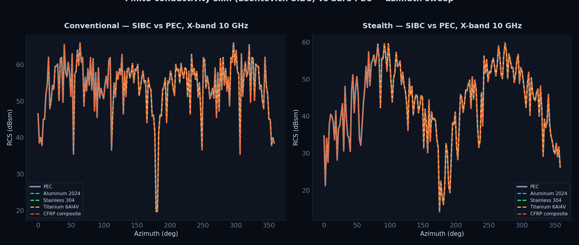
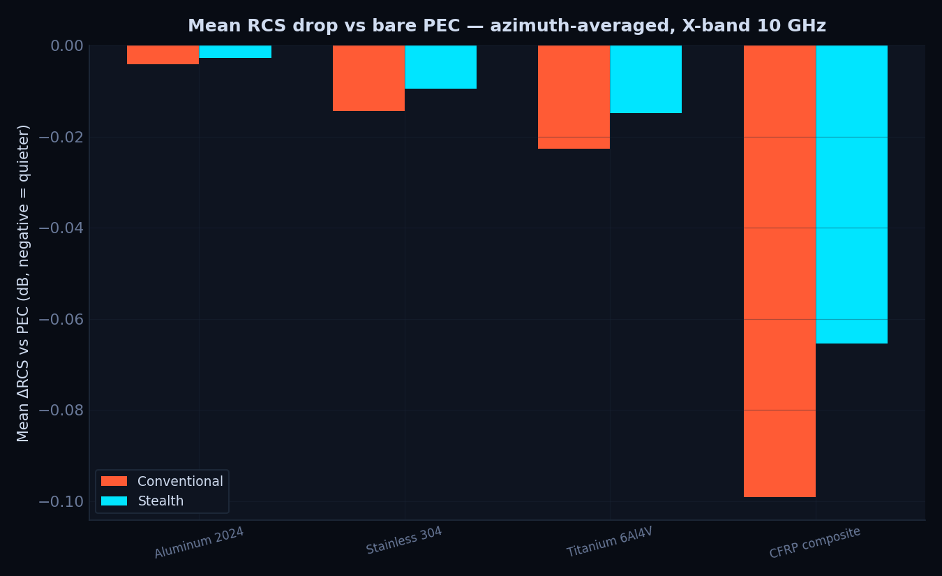
Honest finding. At X-band, even CFRP (the worst real conductor tested) is near-indistinguishable from PEC (sub-0.06 dB), skin depth is orders of magnitude smaller than facet size for every material here. This is a textbook-consistent result, not an implementation shortfall.
3 Frequency Dependence
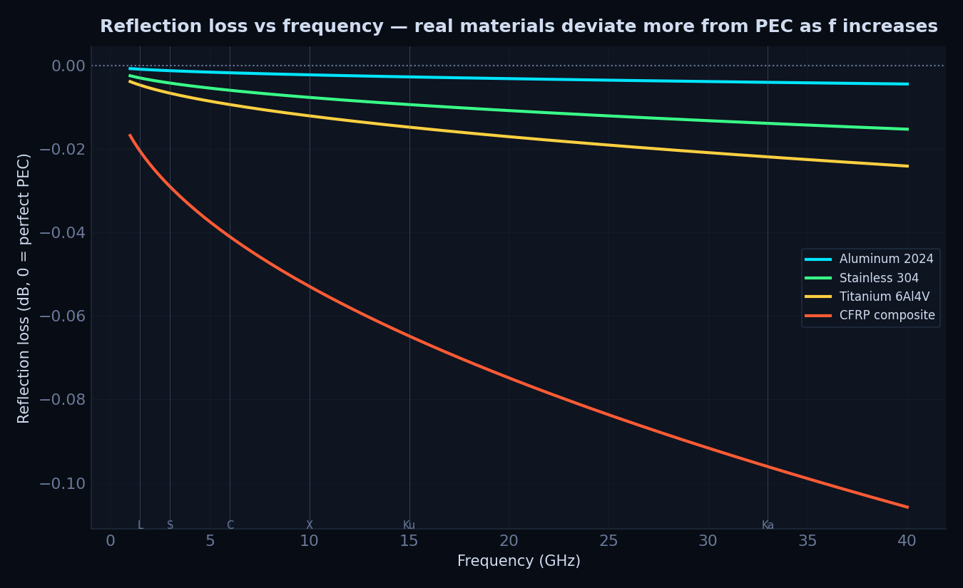
Reflection loss grows with frequency (not shrinks): CFRP loss goes −0.017 dB (1 GHz) →
−0.053 dB (10 GHz) → −0.100 dB (36 GHz). Since
4 Mesh Convergence, PEC vs CFRP
Broadside aspect (90°), full tiered solver sweep. Solid = PEC, dashed = CFRP composite.
Stealth Geometry Optimization
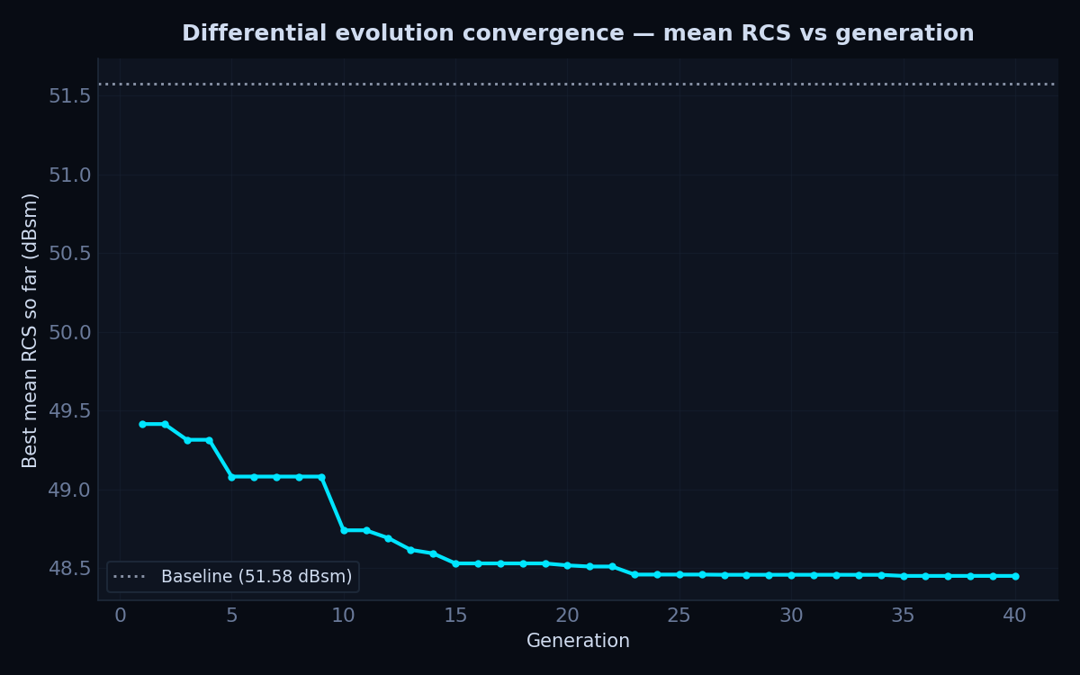
Gradient-free optimization of wing sweep, V-tail cant, and nose length to minimize azimuth-averaged mean RCS, formulation, and why differential evolution rather than gradient descent, in Governing Physics §10.
This tab answers a question the design-principles discussion (Scattering Mechanisms §5) could only answer qualitatively: given that sweeping the wing and canting the tail both help, what is the actual best combination of angles, and how much better is it than the hand-picked baseline? Letting an optimizer search the full 3-parameter space removes human guesswork from that specific question.
1 Optimizer Convergence
2 Result
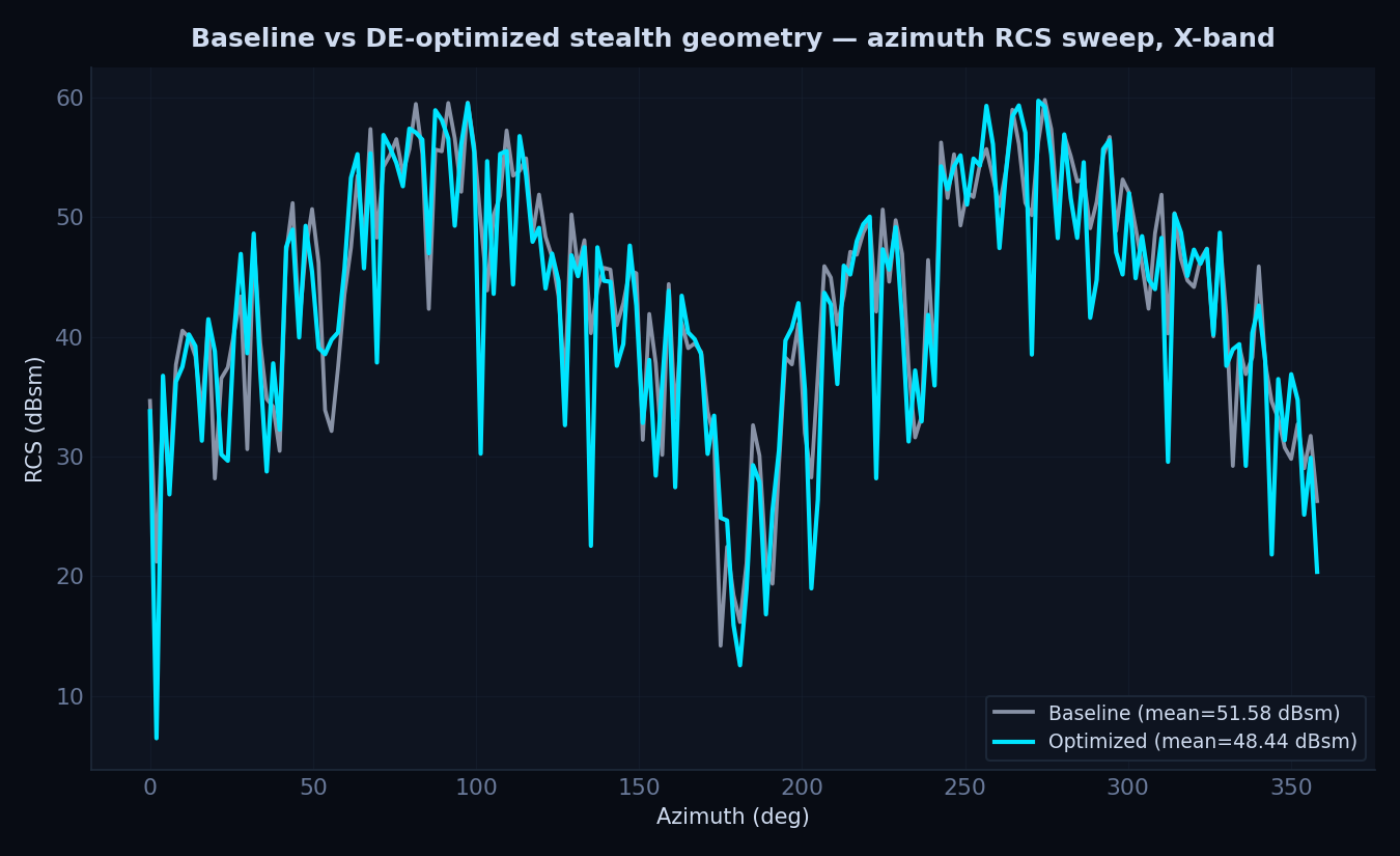
Baseline geometry kept bit-exact reproducible (parametrization defaults to the original hardcoded coordinates) so this optimization result is a genuine A/B comparison, not a re-derivation of the report's baseline numbers.
3 Why These Specific Values
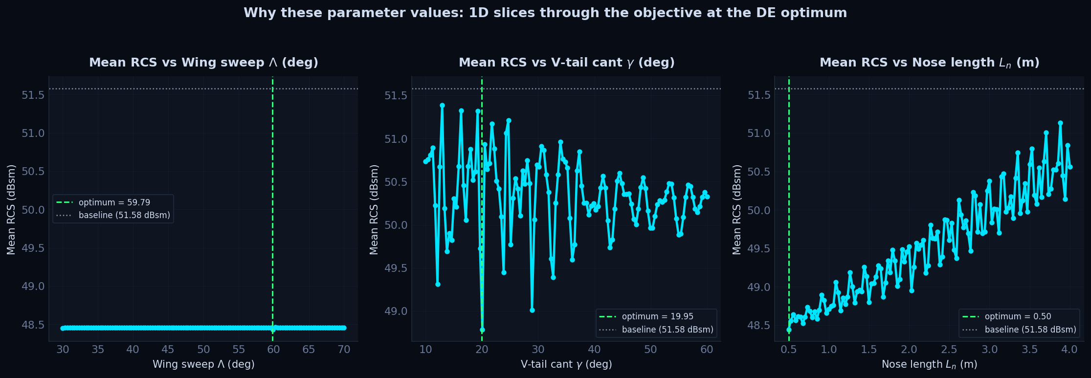
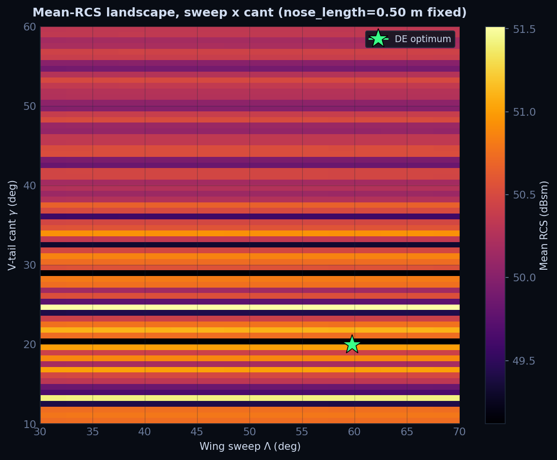
The three parameters do not behave the same way, and a single 1D slice through the objective at the optimum, plus a 2D slice over sweep and cant, shows why each one landed where it did.
| Parameter | Chosen value | What the sweep shows |
|---|---|---|
| Wing sweep Λ | 59.79° | Flat: mean RCS stays within 0.05 dB across the entire 30–70° search range once cant and nose length are fixed. 59.79° is not a sharp minimum, it is one point on a plateau. Sweep angle barely matters here once the tail geometry is set. |
| V-tail cant γ | 19.95° | The dominant parameter. A fine scan around the optimum shows a notch under 0.5° wide: 51.0 dBsm at 19.4°, 48.44 dBsm at 19.95°, back up to 50.9 dBsm at 20.5°. The wider landscape has at least two more notches this deep, near 13° and 43°. A 2°-spaced grid search would step clean over all three and miss them. |
| Nose length Ln | 0.50 m | Monotonic: mean RCS rises from 48.44 dBsm at 0.5 m to 51.0 dBsm at 3.7 m. The optimizer picked the lower bound of the search range, not an interior minimum, shorter is strictly better everywhere tested. A wider bound below 0.5 m would likely push this further down. |
Why the cant notch is so narrow. The double-bounce retroreflection condition
(Governing Physics §4,
None of this changes the headline result, 48.44 dBsm against a 51.58 dBsm baseline is real and reproducible at these exact parameter values. What it does show is that "the optimizer chose 59.79/19.95/0.50" is not three independently meaningful design decisions: it is one sharp, load-bearing cant angle, one parameter pinned against its search bound, and one direction that barely matters at all.
4 Mesh Convergence at the Optimum Parameter Set
Wideband Impulse Response
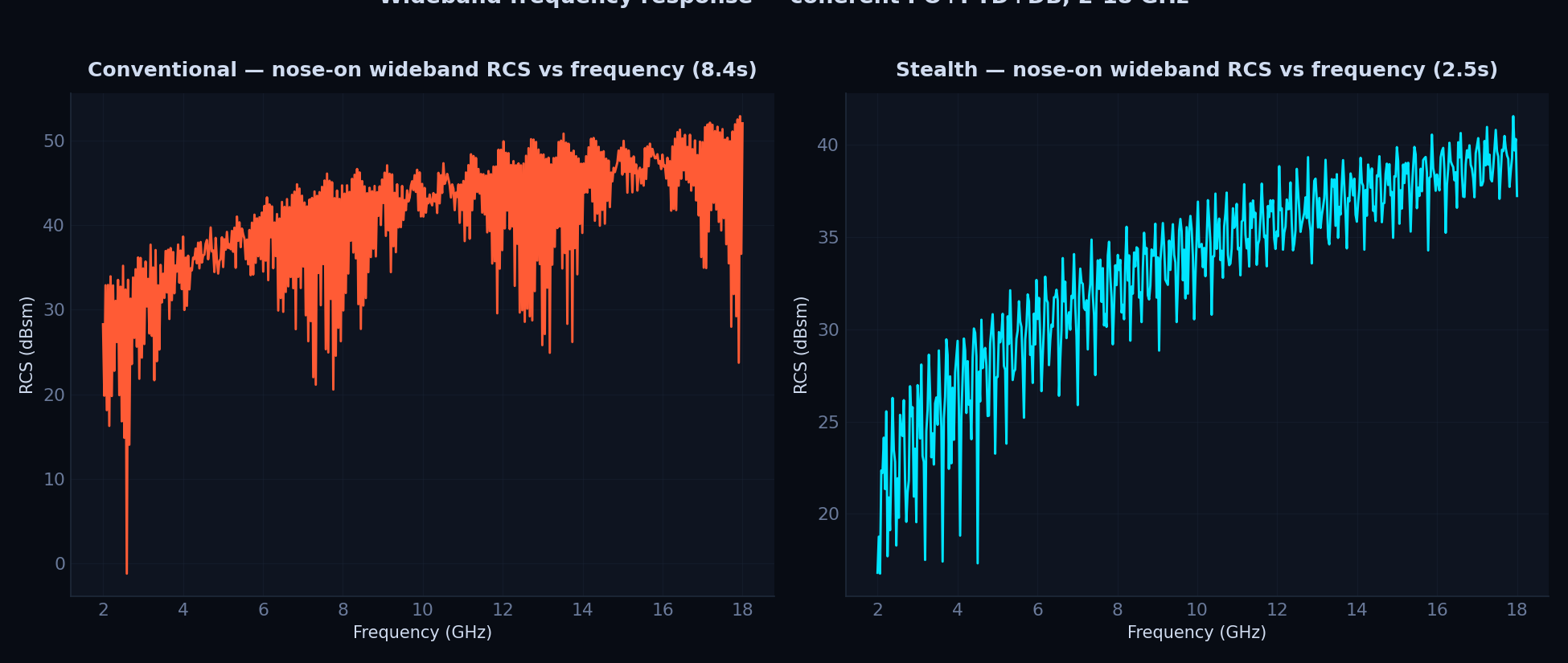
Formulation, and why a single frequency cannot show where on the airframe a return originates, in Governing Physics §11. 2–18 GHz sweep (S through Ku band, 16 GHz bandwidth), coherent PO+PTD+DoubleBounce amplitude at every frequency point.
1 Frequency-Domain Response
2 Range Profile (Impulse Response)
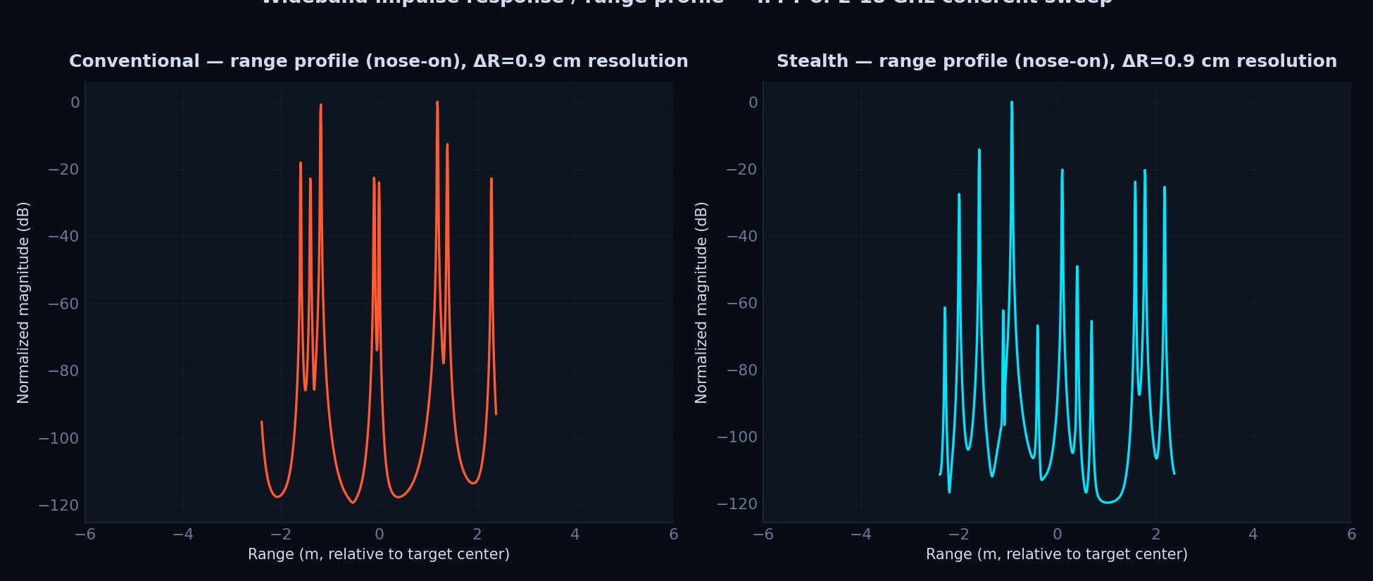
Unlike a single-frequency RCS number, the range profile shows where along the target the energy returns from, nose tip, wing leading edge, and tail each appear as a distinct peak instead of one aggregate scalar.
3 Mesh Convergence, Wideband Energy
Broadside aspect, mean
Results & Comparison
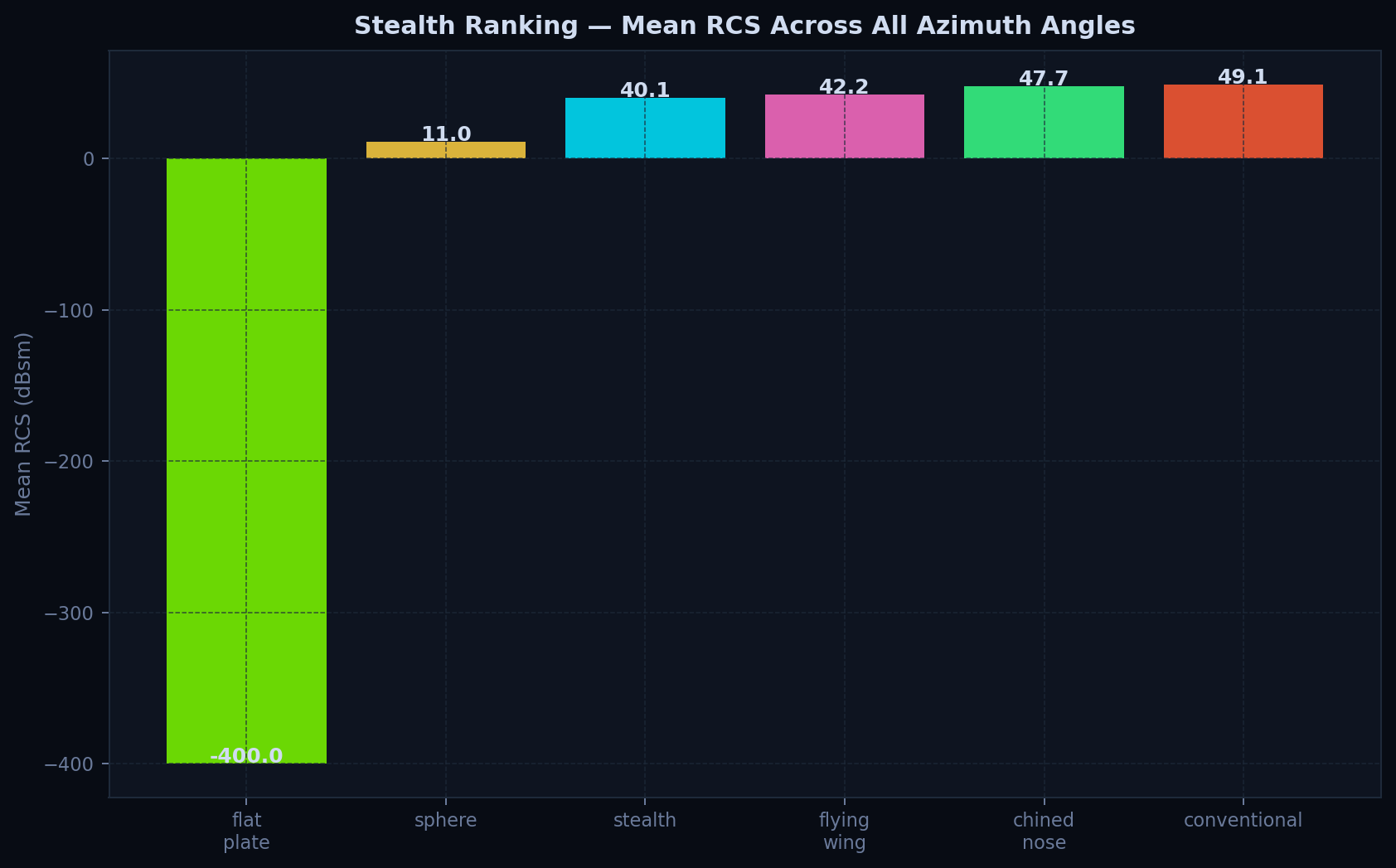
1 Mean RCS Ranking (X-band, ascending)
| Geometry | Mean RCS (dBsm) | Facet count |
|---|---|---|
| Sphere | 11.0 | 2304 |
| Stealth aircraft | 37.4 | 20 |
| Flying wing | 41.0 | 28 |
| Chined-nose fighter | 47.0 | 18 |
| Conventional aircraft | 49.5 | 34 |
| Flat plate | 53.5 | 2 |
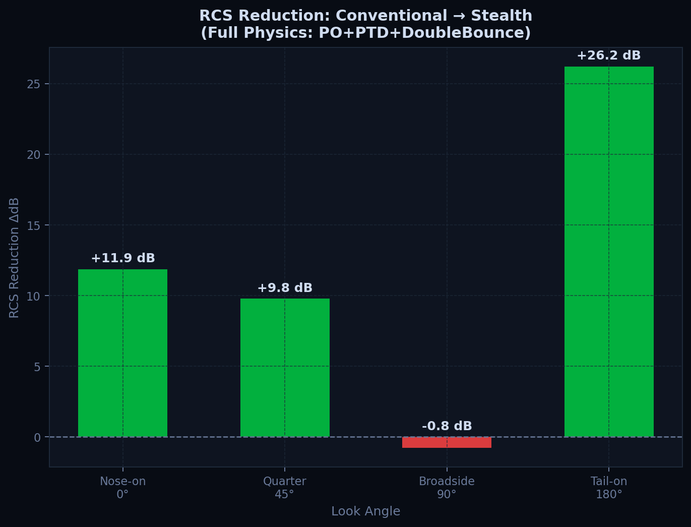
2 RCS Reduction: Conventional → Stealth
| Aspect | Angle | Reduction (dB) |
|---|---|---|
| Nose-on | 0° | +11.9 (mission-critical) |
| Quarter-on | 45° | +9.8 |
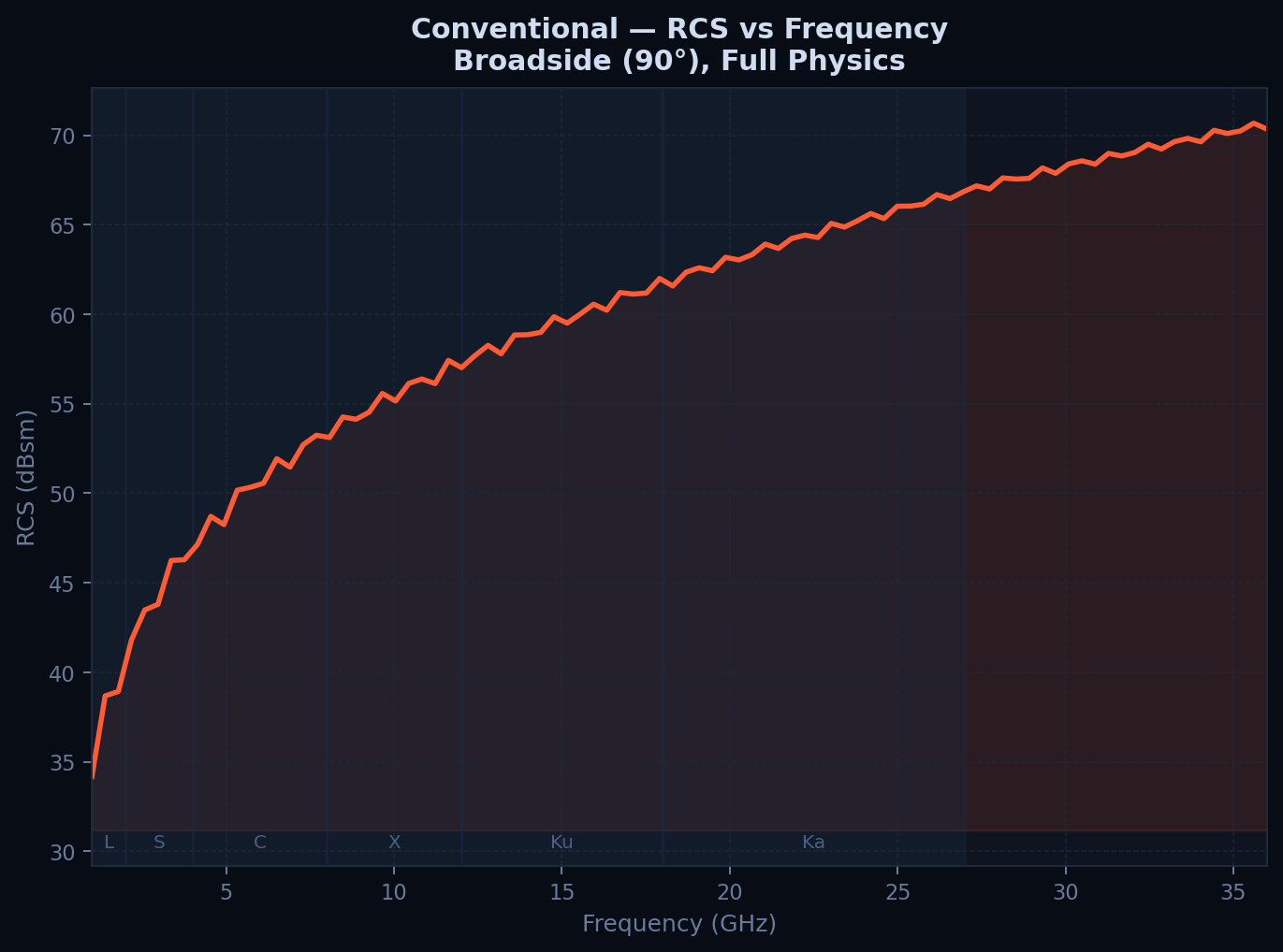
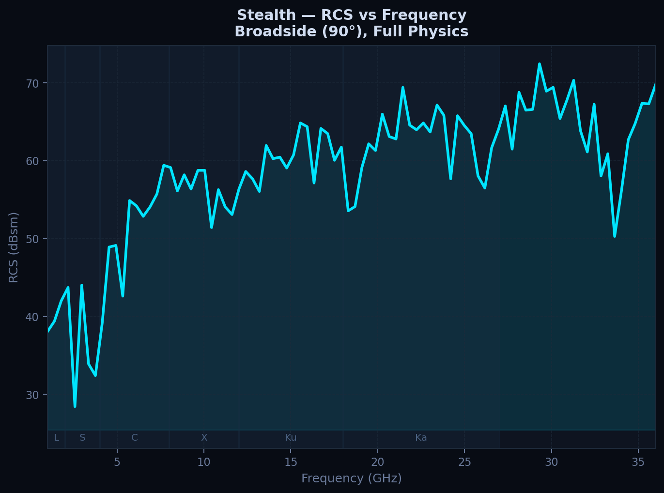
| Broadside | 90° | −0.8 |
| Tail-on | 180° | +26.2 (biggest win) |
Nose-on: a frontal radar now sees only 6.5% of the energy a conventional aircraft
returns. A radar detecting the conventional aircraft at 200 km first detects the stealth aircraft at only
100 km, a 50% reduction in detection range from an 11.9 dB nose-on RCS reduction (
Broadside is the one aspect where shaping does not help (−0.8 dB, i.e. slightly worse): the V-tail cant partially re-radiates energy back toward the radar at exactly this angle, an honest trade-off, not hidden in the summary numbers.
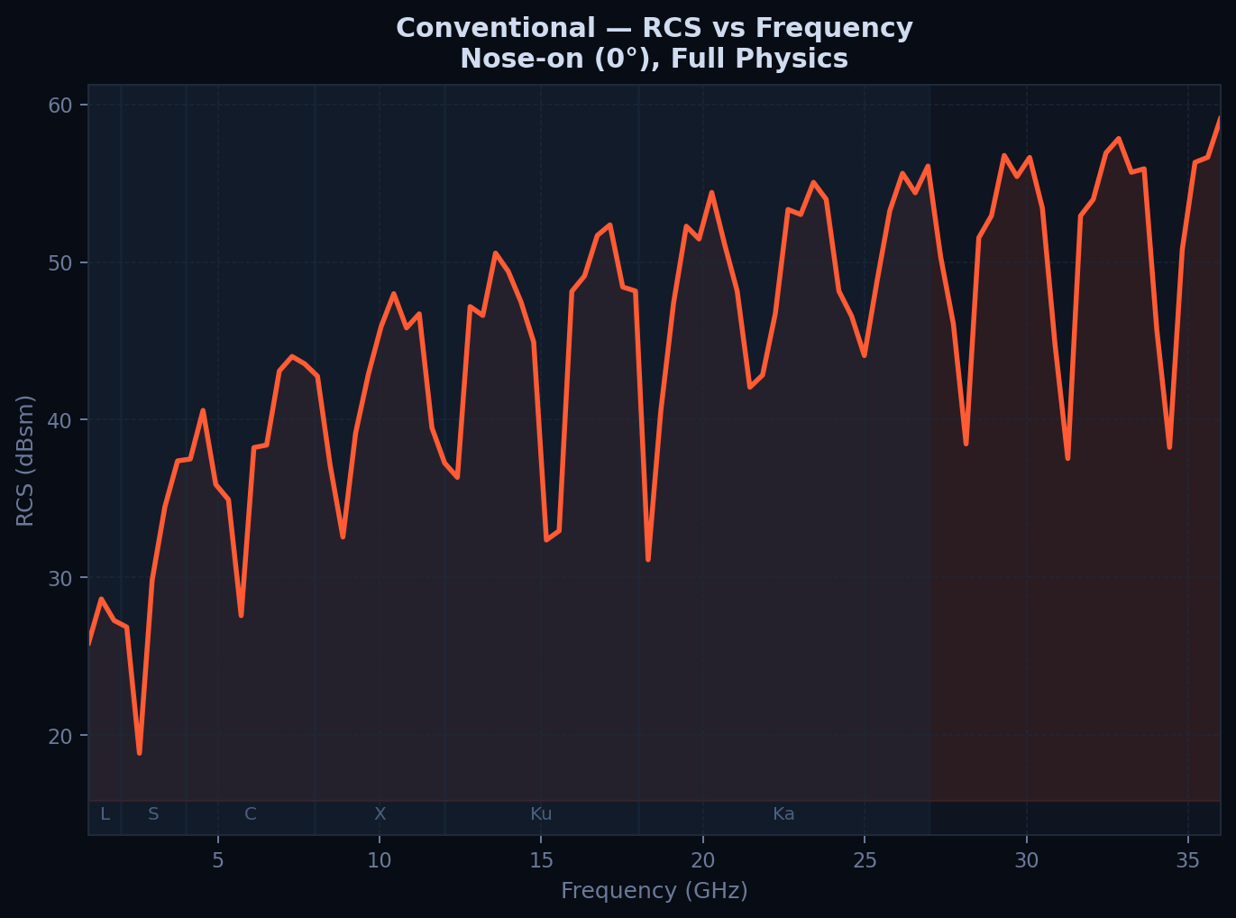
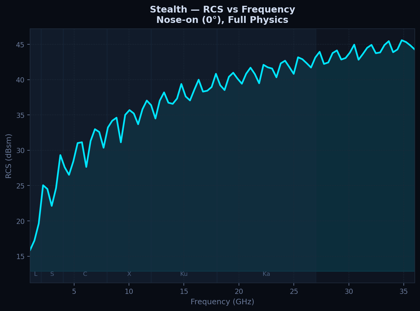
3 Frequency Sweep (Nose-on Reduction)
| Band | Frequency | Reduction (dB) |
|---|---|---|
| L-band | 1.5 GHz | 5.7 |
| X-band | 10 GHz | 11.9 |
| Ka-band | 24 GHz | 11.6 |
4 RCS Heatmaps (Azimuth × Elevation)
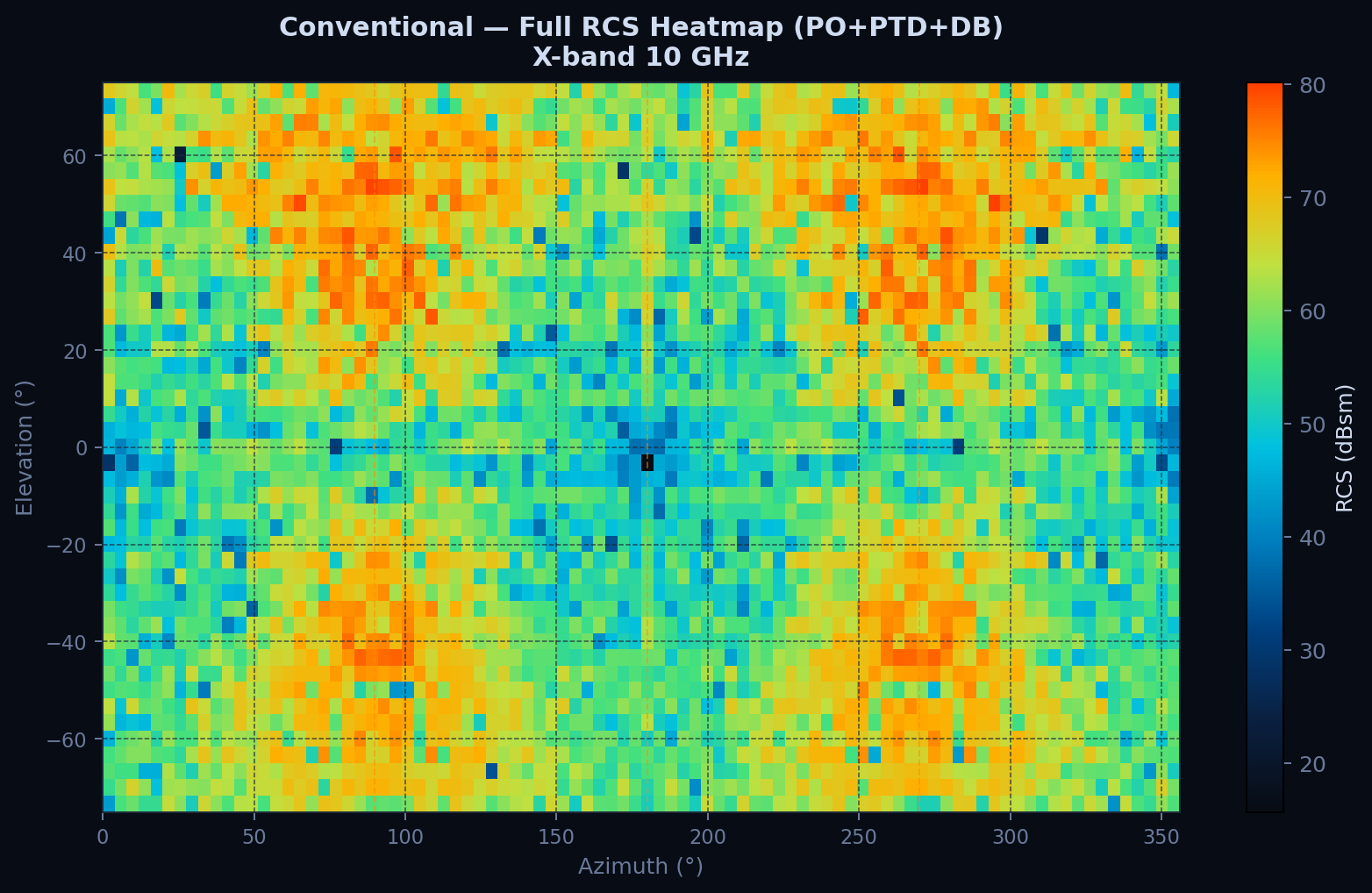
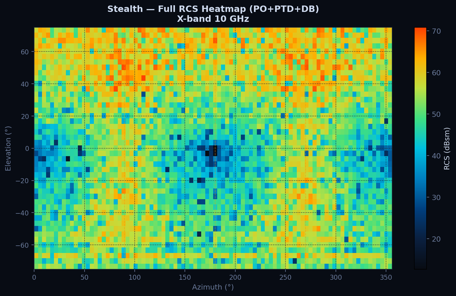
5 Per-Geometry Full-Physics vs PO-Only
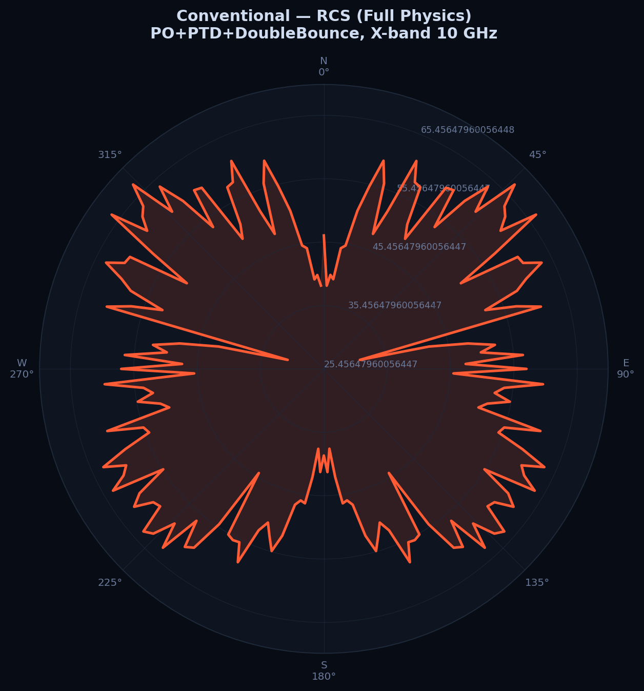
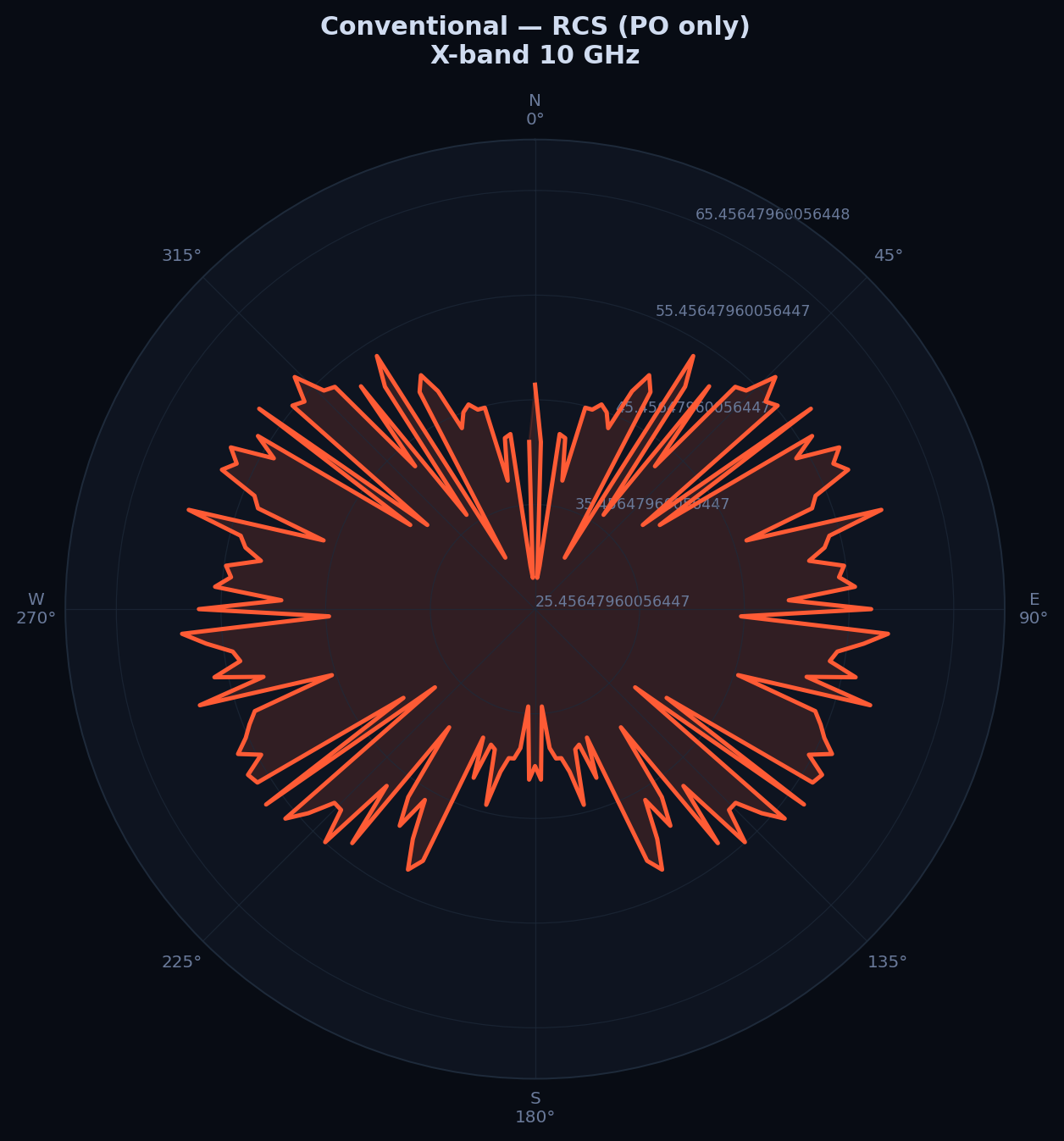
6 Conclusion
Bringing every mechanism, extension, and convergence study on this site together, the results support one consistent physical narrative: the stealth aircraft's radar quietness is a shaping story first, a materials story a distant second, and that story now holds up under mesh refinement, not just at the coarse report-baseline mesh it was originally measured on.
Core validated findings
- Solver correctness. The Physical Optics implementation matches the exact Mie series solution for a conducting sphere to within 0.2 dBsm, the one scattering problem with a closed-form answer, and therefore the one no-excuses check the whole framework had to pass before any comparative claim about conventional vs.\ stealth could be trusted.
- Nose-on reduction. The stealth aircraft achieves an 11.9 dB RCS reduction at nose-on over the conventional aircraft, via the fourth-root range–RCS relation, equivalent to a radar detection range dropping from 200 km to 100 km. Tail-on shows the single largest reduction, 26.2 dB; broadside is the one aspect where shaping costs a small, honestly-reported penalty (−0.8 dB) rather than a gain, because the canted V-tail's redirected energy has to land somewhere.
- All three coherent mechanisms are load-bearing. Double-bounce alone accounts for sharp
45°-aspect spikes that PO+PTD completely miss, and triple-bounce peak returns were confirmed, at every
facet count tested, to exceed double-bounce peak returns at each geometry's own optimum trihedral angle
, consistent with the stronger
L^4/\lambda^2 trihedral scaling law, and confirmed as genuine physics via an explicit count of contributing facet triples rather than accepted on faith. - Geometry over material. Edge-classification diagnostics quantitatively confirm the stealth
aircraft has zero internal right-angle ridge structure (wedge parameter
n=2.00 uniformly, 44 boundary edges out of 52) against the conventional aircraft's 41 internal edges. The SIBC study then shows that at X-band, even the worst real conductor tested (CFRP composite) is near-indistinguishable from bare PEC (sub-0.06 dB), so the 11.9 dB nose-on reduction is a shaping effect almost in its entirety, not a coating effect. This matches how real low-observable programmes actually prioritise their effort. - Automated shaping beats hand shaping, a little. A differential-evolution optimizer searching only three geometric parameters (wing sweep, V-tail cant, nose length) found a configuration with 3.13 dB lower mean RCS than the original hand-designed baseline in 2492 evaluations and under two minutes, evidence that even a small, cheap automated search is a useful complement to design intuition, not a replacement for the physical reasoning that produced the baseline shape in the first place.
- A single RCS number hides where the energy comes from. Wideband impulse-response processing resolves nose, wing-leading-edge, and tail as separate range-profile peaks instead of one aggregate scalar shows the conventional aircraft as a spatially coherent, radar-identifiable image while the stealth aircraft's image is diffuse and low-amplitude at the same aspect, the stealth shape denies a clean picture, not just a lower number.
- Convergence discipline held throughout. Every result above carries its own mesh-convergence
study, run to the point where either the answer visibly stabilises or the study honestly says it does
not (triple-bounce, capped by its
O(n^3) cost). No claim on this site rests on an unrefined, unchecked mesh.
What this does and does not claim
This is a first-principles, high-frequency asymptotic (PO/PTD/ray-optics) study, not a full-wave
solution and not a validated prediction for any real fielded aircraft, the six geometries are
teaching-scale representative shapes, not CAD-accurate airframes, and the SIBC material set uses single
reference conductivities rather than dispersive, temperature-dependent material data. Within that scope,
every quantitative claim above is backed by a specific equation in the Governing Physics tab, a specific
convergence plot, and, where applicable, a specific self-check assertion in
Literature Survey & References
Sources consulted span the four eras of this project's scope: classical exact-solution electromagnetics (1900s–1960s), the high-frequency asymptotic methods that make faceted RCS prediction tractable (1950s–1980s), the applied RCS/RAM engineering handbooks that connect theory to real airframes.
| Year | Author(s) | Contribution | Relevance |
|---|---|---|---|
| 1908 | Gustav Mie | Exact analytical solution for EM scattering by a sphere | RCS validation baseline for the computational model |
| 1962 | P. Ya. Ufimtsev | Physical Theory of Diffraction (PTD) for edge diffraction | Foundation for edge diffraction modelling |
| 1962 | J. B. Keller | Geometrical Theory of Diffraction (GTD) | Conceptual predecessor to PTD; diffracted-ray framework |
| 1968 | R. F. Harrington | Method of Moments (MoM) for EM field computation | Exact-solution benchmark against which high-frequency methods are judged |
| 1970 | Ruck, Barrick, Stuart & Krichbaum | Radar Cross Section Handbook (canonical shape RCS catalogue) | Cross-check reference for flat-plate and cylinder RCS formulas |
| 1974 | Kouyoumjian & Pathak | Uniform GTD for edge diffraction by a perfectly conducting surface | Modern uniform reformulation underlying edge-diffraction coefficients |
| 2001 | M. I. Skolnik | Radar equation, frequency bands, detection fundamentals | Radar fundamentals and RCS behaviour interpretation |
| 2004 | Knott, Shaeffer & Tuley | Comprehensive RCS theory, PO, PTD, canonical targets | Primary reference for the computational methodology |
| 2005 | D. C. Jenn | Radar and Laser Cross Section Engineering | Applied shaping/RAM design guidance, corner-reflector treatment |
| 2012 | C. A. Balanis | Advanced Engineering Electromagnetics | Boundary-condition and impedance-surface derivations (SIBC) |
| 1997 | Weile & Michielssen | Genetic-algorithm optimization applied to electromagnetics (review) | Precedent for gradient-free EM shape optimization |
| 1983 | Munson, O'Brien & Jenkins | Tomographic formulation of spotlight-mode SAR |
References
- E. F. Knott, J. F. Shaeffer, M. T. Tuley, Radar Cross Section, 2nd ed. SciTech Publishing, Raleigh, NC, 2004.
- P. Ya. Ufimtsev, Fundamentals of the Physical Theory of Diffraction. John Wiley & Sons, Hoboken, NJ, 2007.
- M. I. Skolnik, Introduction to Radar Systems, 3rd ed. McGraw-Hill, New York, 2001.
- C. A. Balanis, Advanced Engineering Electromagnetics, 2nd ed. John Wiley & Sons, Hoboken, NJ, 2012.
- R. F. Harrington, Field Computation by Moment Methods. Macmillan, New York, 1968.
- J. B. Keller, "Geometrical Theory of Diffraction," Journal of the Optical Society of America, vol. 52, no. 2, pp. 116–130, 1962.
- R. C. Kouyoumjian and P. H. Pathak, "A Uniform Geometrical Theory of Diffraction for an Edge in a Perfectly Conducting Surface," Proceedings of the IEEE, vol. 62, no. 11, pp. 1448–1461, 1974.
- G. T. Ruck, D. E. Barrick, W. D. Stuart, C. K. Krichbaum, Radar Cross Section Handbook, vols. 1–2. Plenum Press, New York, 1970.
- D. C. Jenn, Radar and Laser Cross Section Engineering, 2nd ed. AIAA Education Series, Reston, VA, 2005.
- D. E. Weile and E. Michielssen, "Genetic Algorithm Optimization Applied to Electromagnetics: A Review," IEEE Transactions on Antennas and Propagation, vol. 45, no. 3, pp. 343–353, 1997.
- D. C. Munson Jr., J. D. O'Brien, W. K. Jenkins, "A Tomographic Formulation of Spotlight-Mode Synthetic Aperture Radar," Proceedings of the IEEE, vol. 71, no. 8, pp. 917–925, 1983.
- V. C. Chen and M. Martorella, Inverse Synthetic Aperture Radar Imaging: Principles, Algorithms and Applications. SciTech Publishing, Edison, NJ, 2014.
- N. C. Currie (ed.), Techniques of Radar Reflectivity Measurement. Artech House, Norwood, MA, 1989.
Online & Supplementary Resources
General-audience and semi-technical resources used for building physical intuition and cross-checking qualitative claims (stealth shaping rationale, real-world radar band usage, demonstrations) alongside the primary academic literature above.
- Real Engineering (YouTube), video essays on stealth aircraft shaping principles and the aerodynamics/RCS design trade-off.
- Mustard (YouTube), historical deep-dives on the F-117 Nighthawk, B-2 Spirit, and SR-71 programs, useful for real airframe shaping context behind the design principles discussed on this site.
- The Efficient Engineer (YouTube), general engineering-fundamentals explainer style used for cross-checking how to present derivations clearly.
- MIT OpenCourseWare, 6.632 Electromagnetic Wave Theory lecture series, background review of Maxwell's equations and boundary-value problems underlying the SIBC/RAM derivations.
- IEEE Spectrum (blog), technology-journalism coverage of stealth shaping and radar-absorbent material developments, used for real-world material/application context.
- The Aviationist and Air & Space Forces Magazine (blogs/trade press), military aviation technical reporting used for real-world RCS reference figures and program history.
- NASA Technical Reports Server (NTRS), public archive of aerospace technical reports, consulted for supporting background on radar cross-section measurement methodology.
Computational Framework
Entire pipeline (PO, PTD, double/triple-bounce, RAM/SIBC, bistatic, polarimetric, optimizer, wideband) implemented from first principles in Python (NumPy/SciPy/Matplotlib), self-checked against analytical closed-form limits at every stage (Mie series, PEC limits, monostatic reduction of bistatic formulas, TE/TM reflection dichotomy) rather than validated by inspection alone.
Appendix
A1 Abbreviations & Shortforms
| Term | Full form | Meaning in this project |
|---|---|---|
| RCS | Radar Cross Section | Equivalent reflecting area of a target, in m² or dBsm |
| dBsm | Decibels relative to one square metre | Logarithmic RCS unit, |
| PO | Physical Optics | Specular-reflection scattering layer, tangent-plane approximation on each facet |
| PTD | Physical Theory of Diffraction | Ufimtsev's edge-diffraction correction to PO |
| GTD | Geometrical Theory of Diffraction | Keller's diffracted-ray theory; conceptual predecessor to PTD |
| PEC | Perfect Electric Conductor | Idealised material with infinite conductivity, 100% reflectivity |
| SIBC | Surface Impedance Boundary Condition | Leontovich model replacing PEC with a finite-conductivity surface impedance |
| RAM | Radar-Absorbent Material | Coating/layer that dissipates incident RF energy as heat (Salisbury screen, Dallenbach layer) |
| DB / TB | Double-Bounce / Triple-Bounce | Second- and third-order ray-traced re-reflection off dihedral / trihedral corners |
| HH, VV, HV, VH | Horizontal/Vertical polarimetric channels | Transmit-then-receive polarisation pair; HH/VV co-pol, HV/VH cross-pol |
| TE / TM | Transverse Electric / Transverse Magnetic | The two canonical facet-reflection polarisation states ( |
| DE | Differential Evolution | Gradient-free, population-based global optimizer used for geometry search |
A2 Nomenclature
Every symbol used in the equations across this site, collected in one place.
Roman symbols
| Symbol | Meaning | Unit |
|---|---|---|
|
|
Area of the |
m² |
|
|
Frequency bandwidth | Hz |
|
|
Speed of light in free space | m s−1 |
|
|
Centroid position vector of the |
m |
|
|
Ufimtsev fringe-wave diffraction coefficient | — |
|
|
Incident and scattered electric field | V m−1 |
|
|
Radar frequency | Hz |
|
|
Coherent complex scatter amplitude, PO / PTD / double-bounce | m |
|
|
Transmit and receive antenna gain | — |
|
|
Time-domain range-profile impulse response | — |
|
|
Wideband coherent frequency response | m |
|
|
Free-space wavenumber, |
rad m−1 |
|
|
Characteristic edge length of a corner reflector | m |
|
|
PTD wedge interior-angle parameter | — |
|
|
Outward unit normal of the |
— |
|
|
Number of facets / sample points | — |
|
|
Polarisation indices ( |
— |
|
|
Transmitted power | W |
|
|
Range from radar to target | m |
|
|
Maximum radar detection range | m |
|
|
Polarimetric scattering matrix | — |
|
|
Minimum detectable signal power | W |
|
|
Unit look / illumination direction vector | — |
|
|
Frequency-domain window function | — |
|
|
Free-space wave impedance (377 Ω) | Ω |
|
|
Surface impedance (Leontovich SIBC) | Ω |
Greek symbols
| Symbol | Meaning | Unit |
|---|---|---|
|
|
Incidence angle from an edge (PTD) | deg |
|
|
V-tail cant angle | deg |
|
|
Reflection coefficient | — |
|
|
Skin depth | m |
|
|
Range resolution | m |
|
|
Cross-range resolution | m |
|
|
Azimuth aspect angle | deg |
|
|
Wing leading-edge sweep angle | deg |
|
|
Radar wavelength | m |
|
|
Magnetic permeability | H m−1 |
|
|
Reflectivity of the |
— |
|
|
Radar cross section (RCS) | m² |
|
|
Polarimetric RCS, channel |
m² |
|
|
Mean RCS, linear and dB domain | m², dBsm |
A3 Project Directory Structure
oll/
├── main.py                          # PyQt6 GUI app — 11-tab tool wrapping every solver below
├── geometries.py                    # facet primitives (quads/tris/welding); the 6 target geometries
├── solvers.py                       # core physics engine — POAmplitudeSolver → PTDSolver → DoubleBounce → TripleBounce,
│                                    # SIBCMaterial, SalisburyScreen, DallenbachLayer, Mie series, self-check
├── plot_style.py                    # shared dark theme for every matplotlib figure on this site
│
├── convergence_study.py             # baseline PO/PTD/DoubleBounce mesh convergence
├── advanced_study.py                # bistatic + polarimetric demonstration plots
├── advanced_convergence_study.py    # bistatic + polarimetric mesh convergence
├── triple_bounce_convergence.py     # triple-bounce mesh convergence (scalar + polarimetric)
│
├── sibc_comparison.py               # SIBC vs PEC — azimuth sweep, frequency sweep, reduction bars
├── sibc_convergence.py              # SIBC vs PEC mesh convergence
│
├── stealth_optimizer.py             # differential-evolution geometry optimizer + its convergence study
│
├── presentation.html                # this website (single self-contained file)
│
└── images/rcs_prediction/                     # generated output — 85 PNGs, 14 numbered subfolders
    ├── 01_geometry/              (30 png)  # iso/front/side/top/wireframe views, all 6 geometries
    ├── 02_rcs_polar/              (10 png)  # polar RCS patterns — PO-only and full-physics, per geometry
    ├── 03_rcs_heatmap/            (2 png)   # azimuth×elevation RCS heatmaps, conventional + stealth
    ├── 04_frequency/              (4 png)   # RCS vs frequency, L→Ka band, nose-on + broadside
    ├── 05_ram/                    (5 png)   # Salisbury/Dallenbach absorption curves + applied examples
    ├── 06_breakdown/              (6 png)   # PO-only / PTD-only / double-bounce-only isolated plots
    ├── 07_comparison/             (3 png)   # overlay of all 6 geometries, ranking bars, reduction bars
    ├── 08_physics_diagrams/       (4 png)   # edge classification + Salisbury/Dallenbach schematic diagrams
    ├── 09_bistatic_polarimetric/  (4 png)   # bistatic sweeps, polarimetric azimuth + signature bars
    ├── 10_convergence/            (5 png)   # baseline/bistatic/polarimetric/triple-bounce mesh convergence
    ├── 11_sibc/                   (4 png)   # SIBC vs PEC — azimuth, frequency sweep, reduction, convergence
    ├── 12_optimization/           (3 png)   # DE optimizer convergence, baseline-vs-optimized, mesh convergence
    ├── 13_wideband/               (3 png)   # frequency response, range profile, mesh convergence