rockmoc · rocket nozzle design with MOC

What this is

A NOZZLE DESIGN LAB
IN A PYTHON PACKAGE

Most student “nozzle codes” stop at a cone or a single MLN sketch. rockmoc is the toolkit I wished I had: several real contour families, honest performance estimates, plots you can drop into a report, and checks against NASA/NACA/textbook numbers so you know the code is not inventing physics.

You describe the gas (γ and R, or a teaching preset like LOX/RP-1), the throat radius, and exactly one expansion target — exit Mach, area ratio, or pe/pc. A designer function marches the method of characteristics and returns a wall polyline plus metrics.

From there you can export CSV for CAD, plot a dark dashboard, compare families side by side, or run the production pipeline (finer mesh, optional multi-γ, boundary-layer growth, field C_F, altitude sweep).

Library API + optional CLI (rockmoc design …)
SI meters; throat at x = 0, r = R_t
Perfect gas, multi-γ tables, optional CEA/Cantera
Student reports, notebooks, homework set
Deep validation with reference vs solver + error %
MIT licensed · no GPU · works offline once installed

What it can do

SIX PILLARS OF THE TOOLKIT

Everything is aimed at the same loop: design → inspect → export → defend the numbers.

Design

Contours that match textbooks

Planar NASA MLN, axisymmetric MLN, ideal, TIC, Rao TOP/TOC, a 15° cone baseline, and Lee/Vernacchia aerospikes (full, truncated, with cowl).

Accuracy

Production pipeline

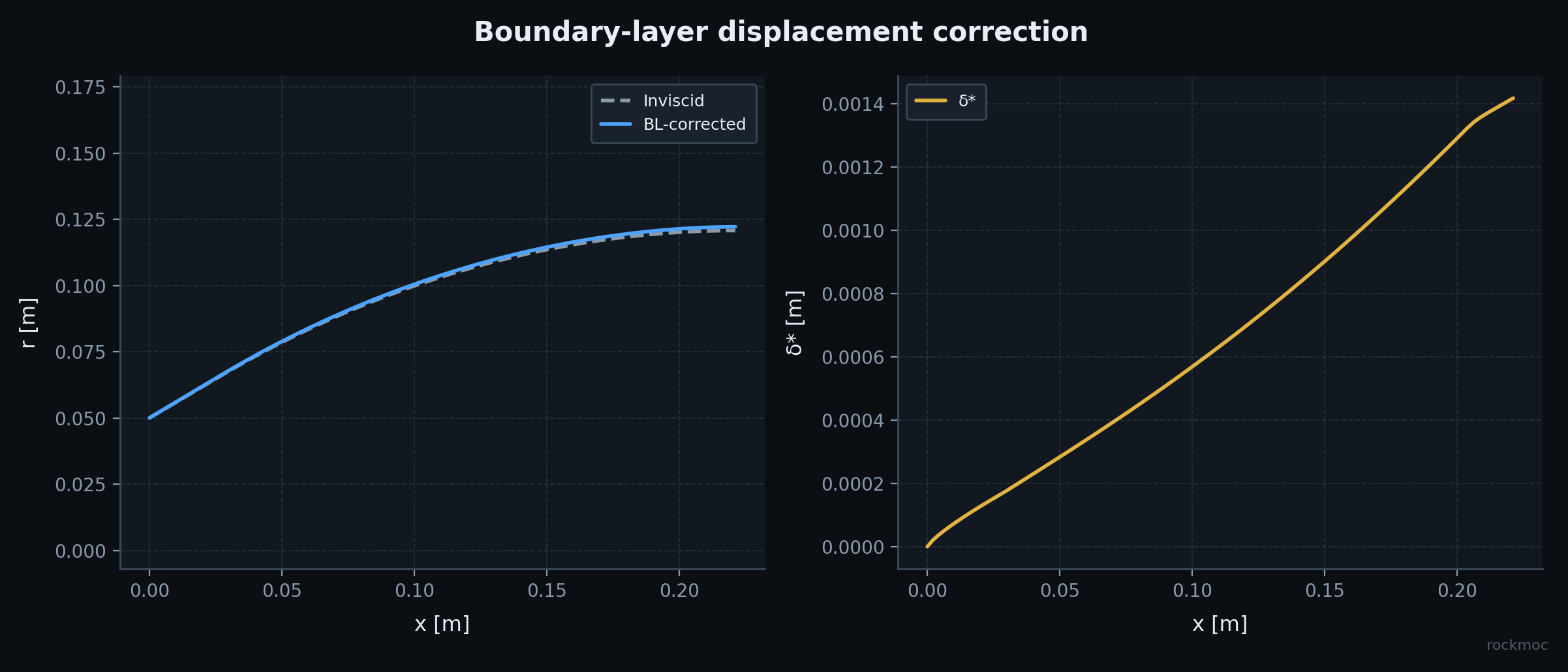
One call chains fine MOC, expansion tables, Sauer-style throat start, BL δ*, exit-plane C_F, altitude sweep, and optional mesh certificates.

Analysis

Performance & trades

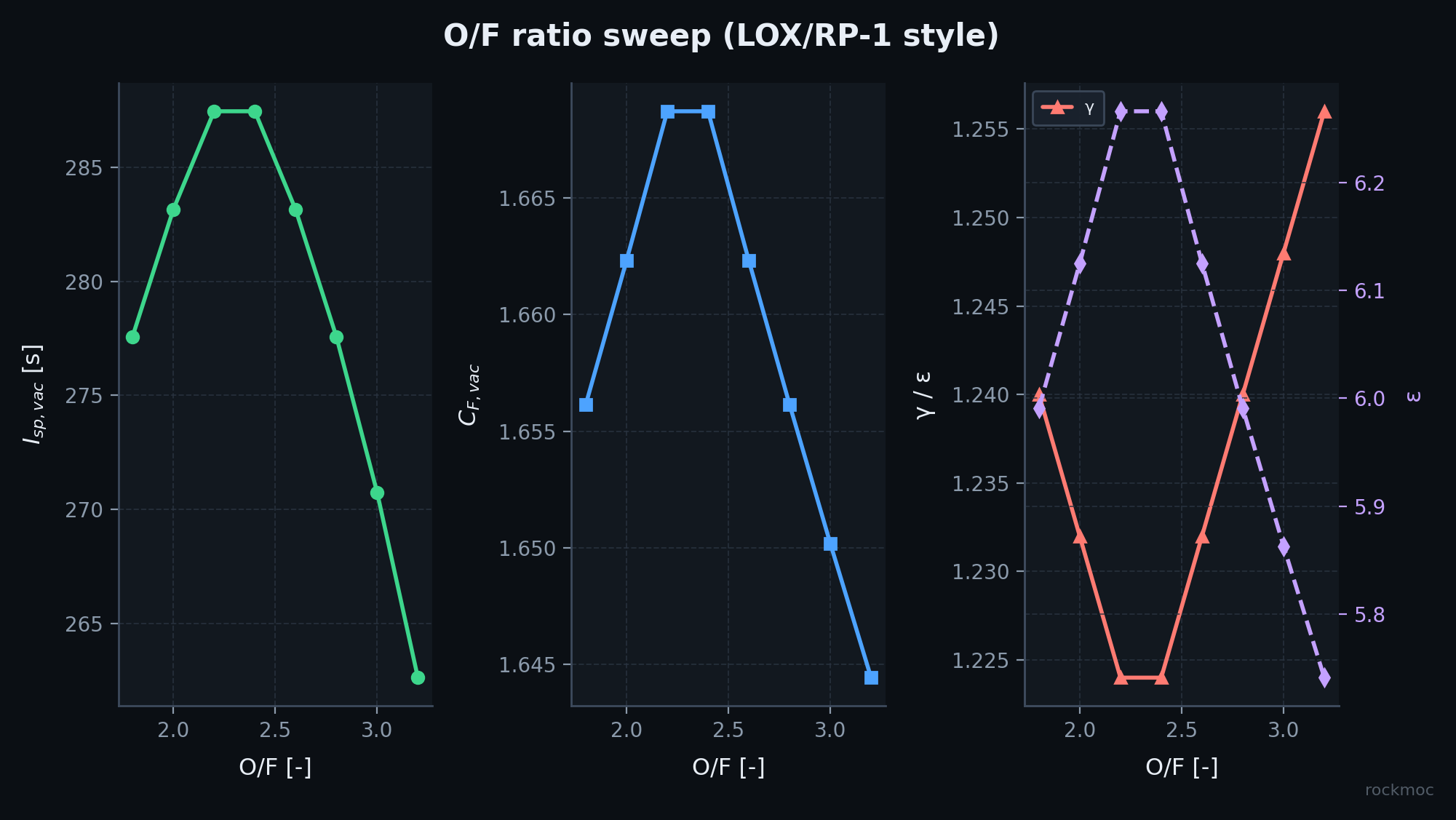
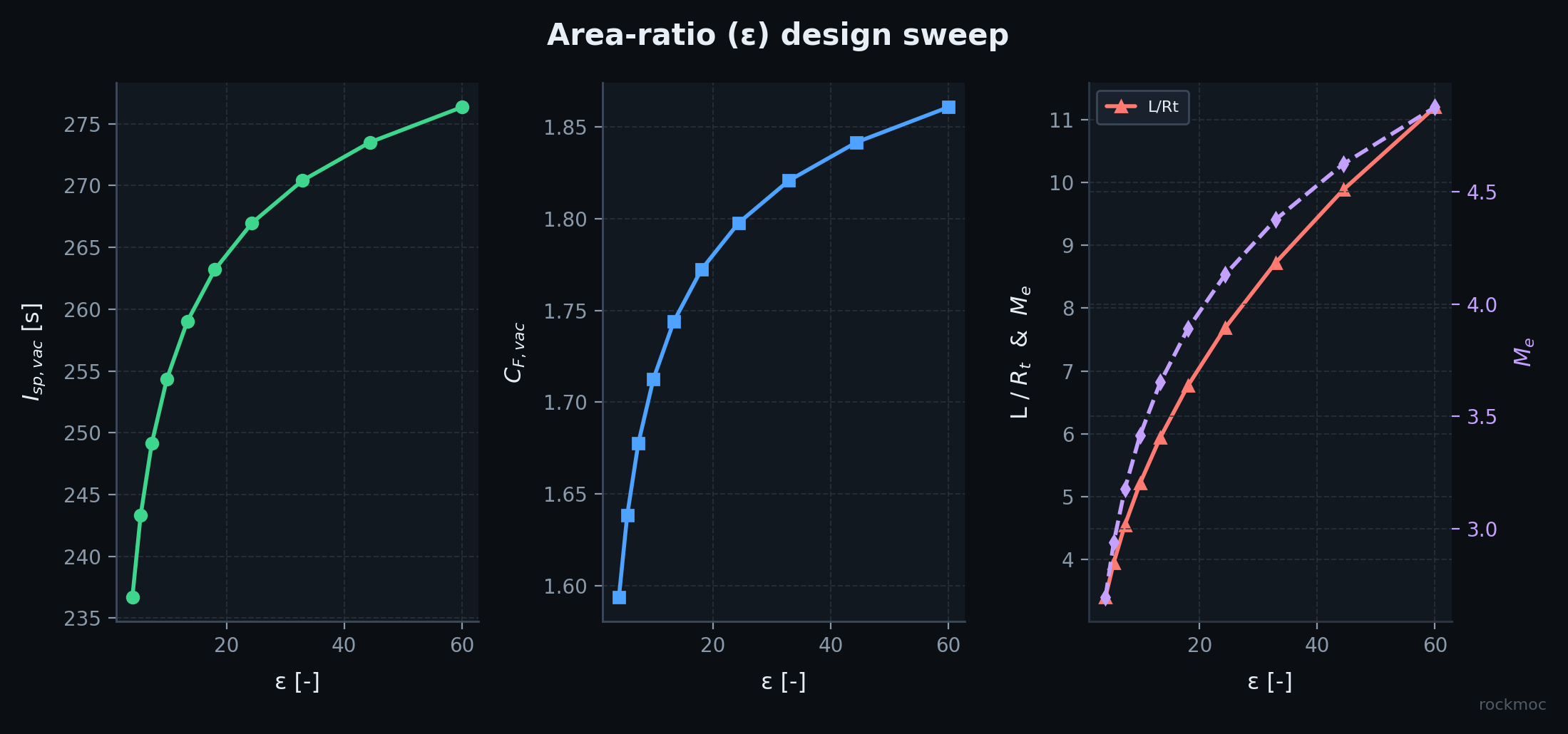
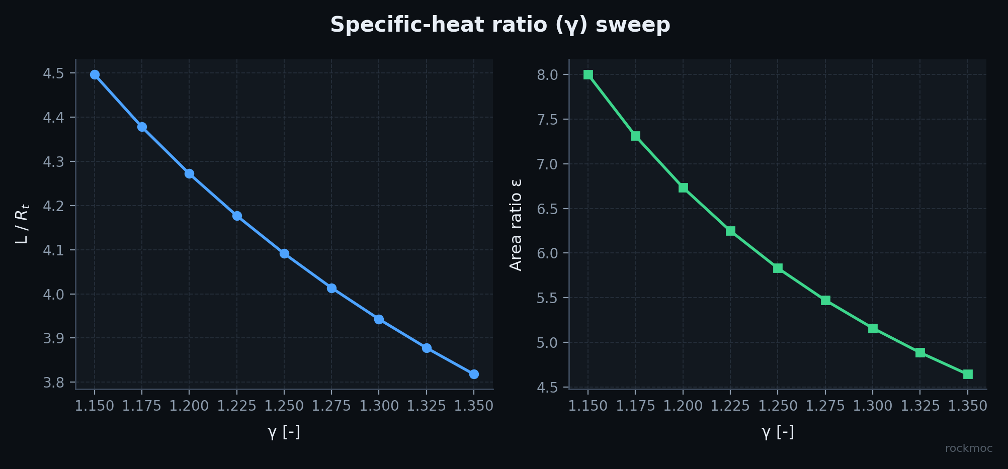
Vacuum and ambient C_F / I_sp, divergence efficiency, O/F–γ–ε sweeps, and fair comparisons you can paste as Markdown or LaTeX tables.

Thermo

Gases that fit the job

Constant-γ perfect gas, multi-γ tables along Mach, teaching presets, and optional RocketCEA frozen chemistry for more realistic γ and R.

Plots

Figures for reports

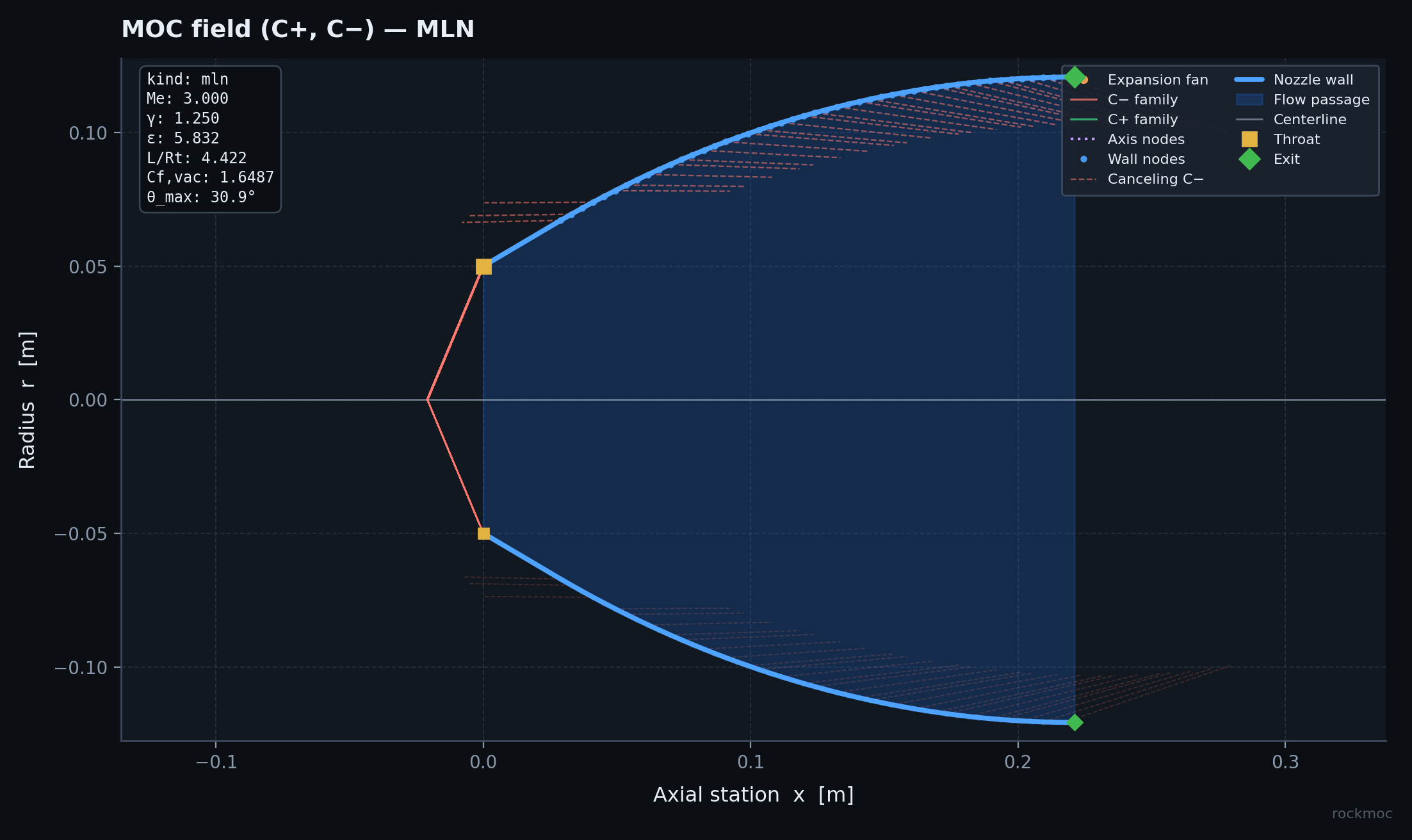
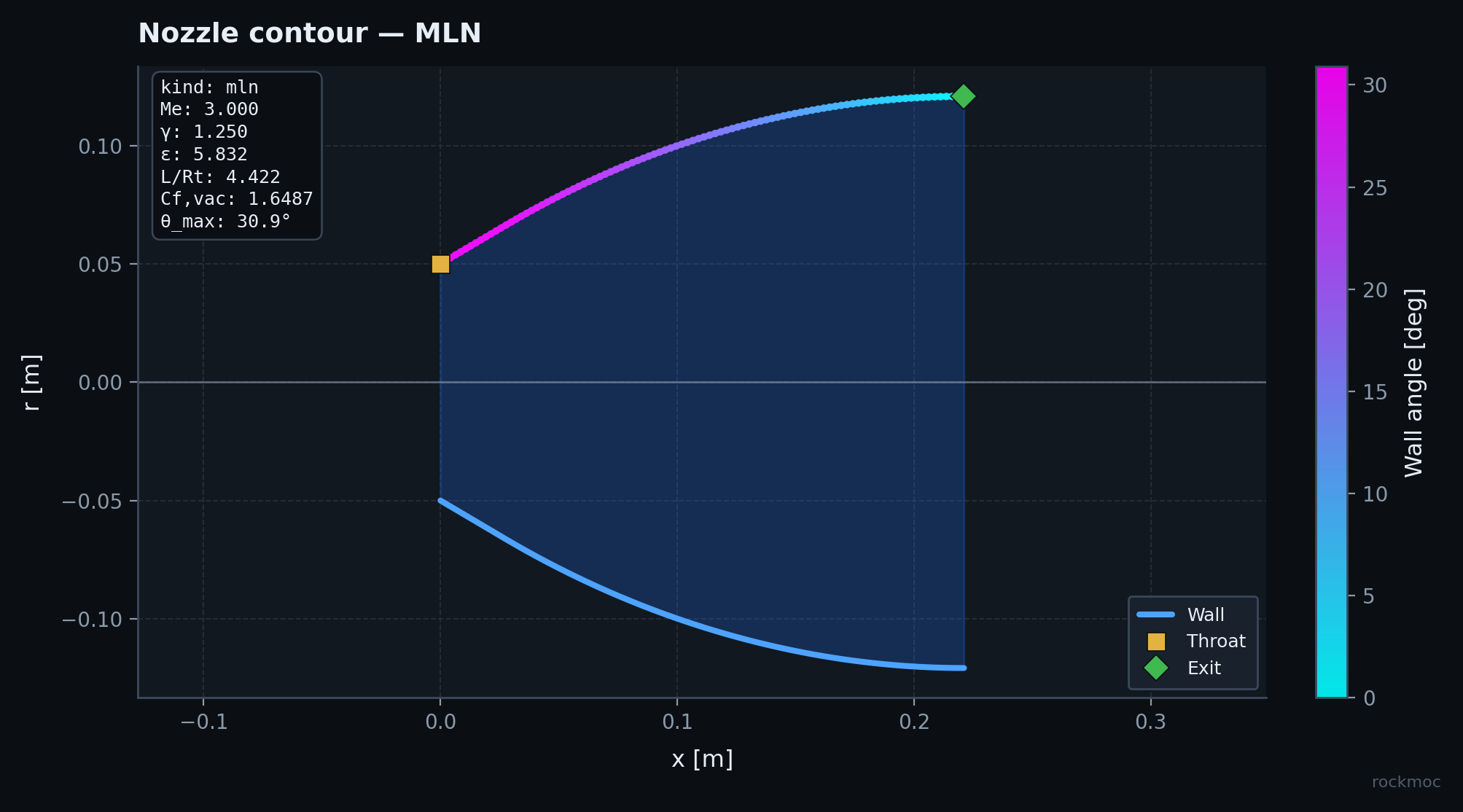
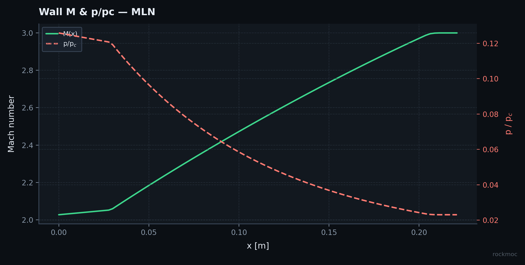
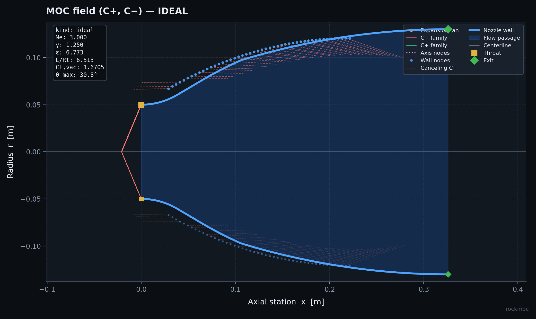
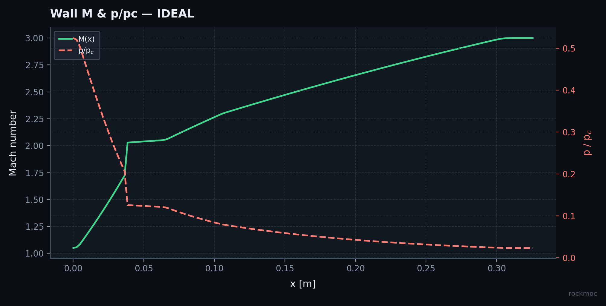
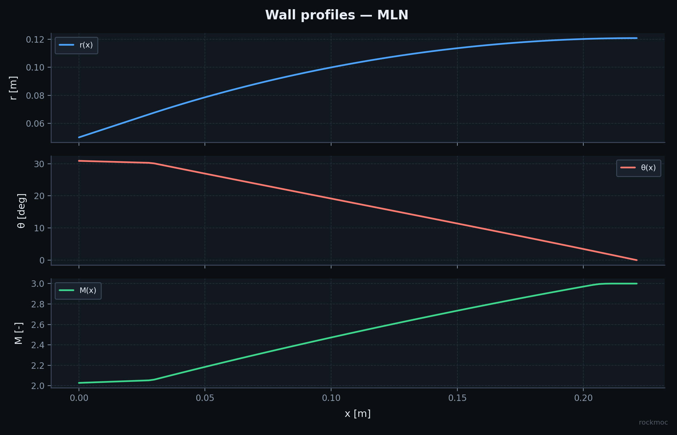
Post-solve dashboards: wall, MOC field with C+/C−, profiles, edge M and p/p_c, altitude, BL, aerospike — dark theme, optional PNG save.

Students

Course-friendly UX

Errors that say how to fix them, unit-aware reports, lab-report generator, glossary, worked problems, and four Jupyter tutorials.

Nozzle families

PICK THE SHAPE THAT MATCHES
THE QUESTION YOU ARE ASKING

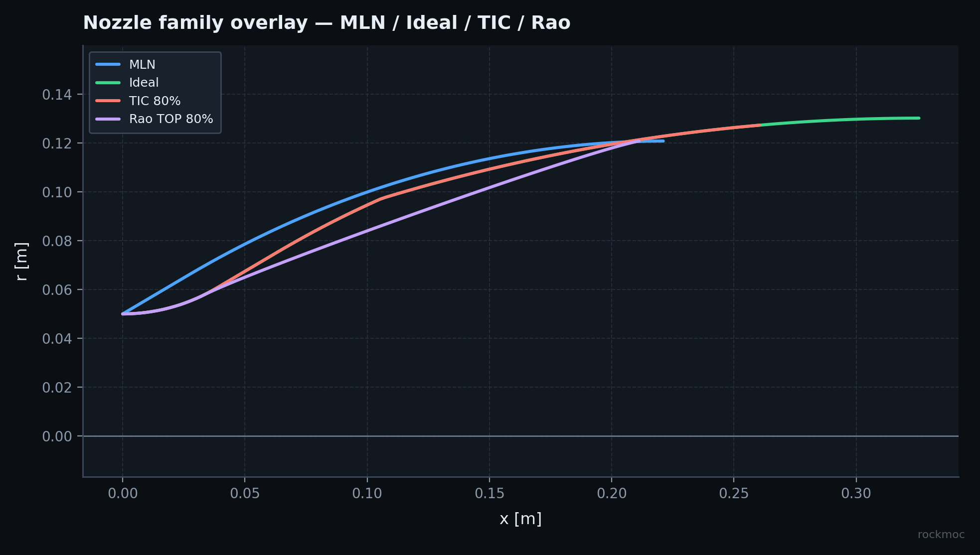
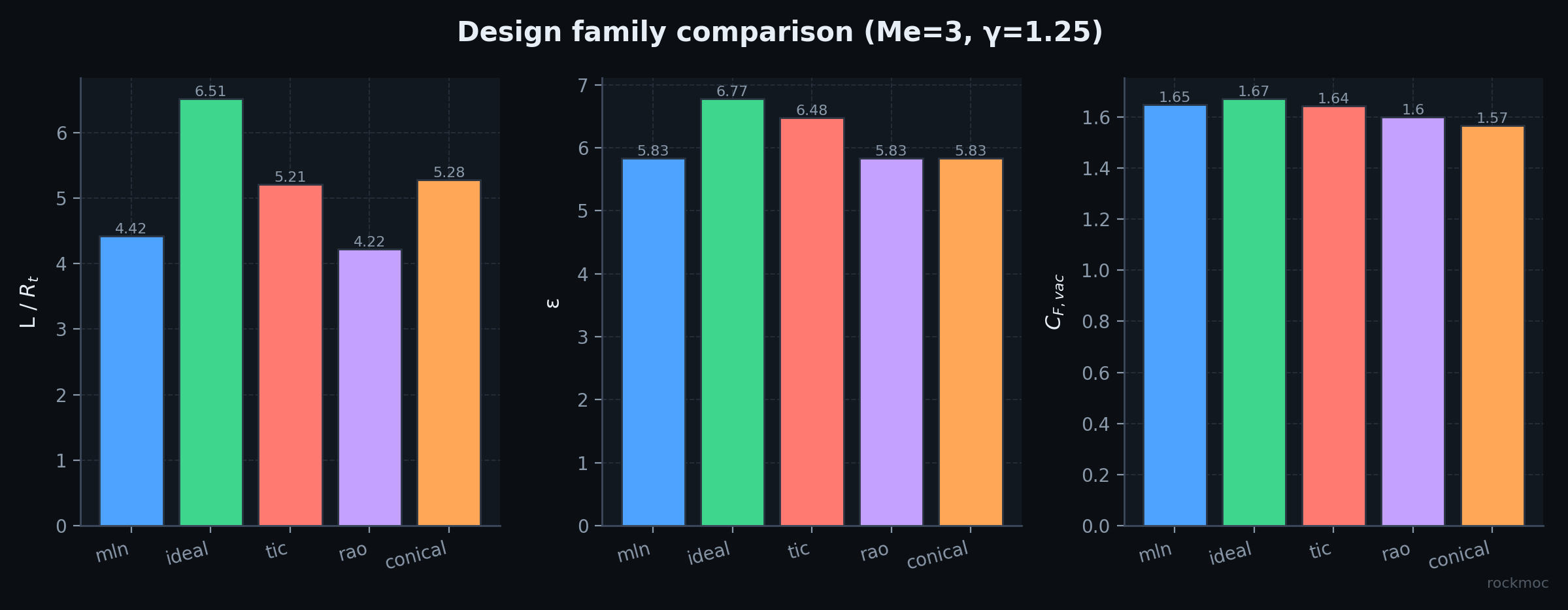
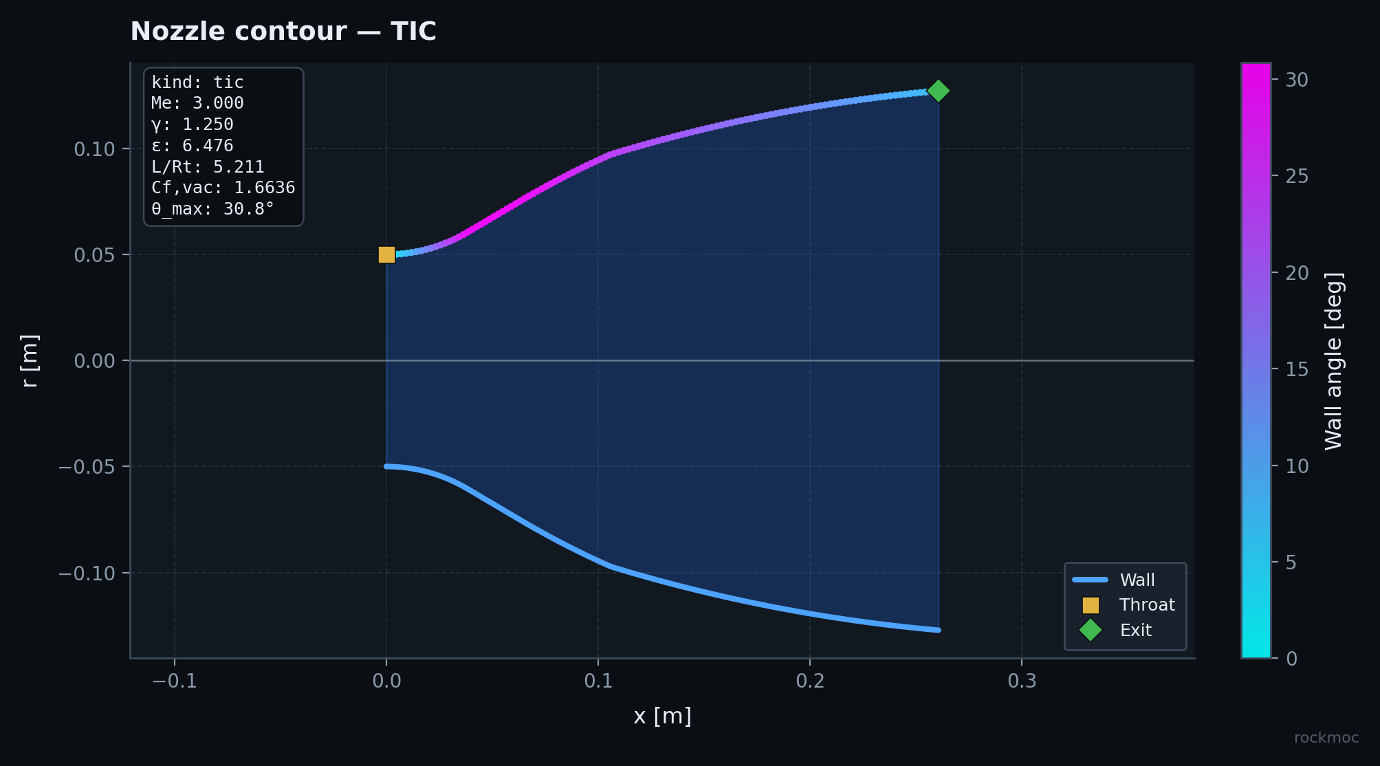
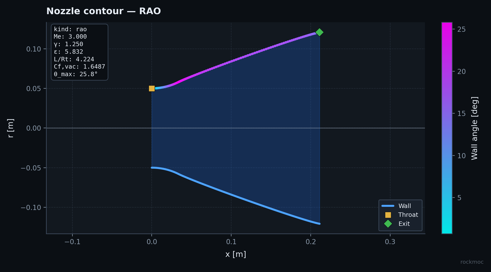
Same Me, γ, and throat — different designers. A typical length story is MLN shorter than Rao TOP (~80% of a 15° cone), TIC somewhere in the middle of ideal, and a plain cone as the honest baseline every textbook still uses.

MLN

Minimum-length nozzle

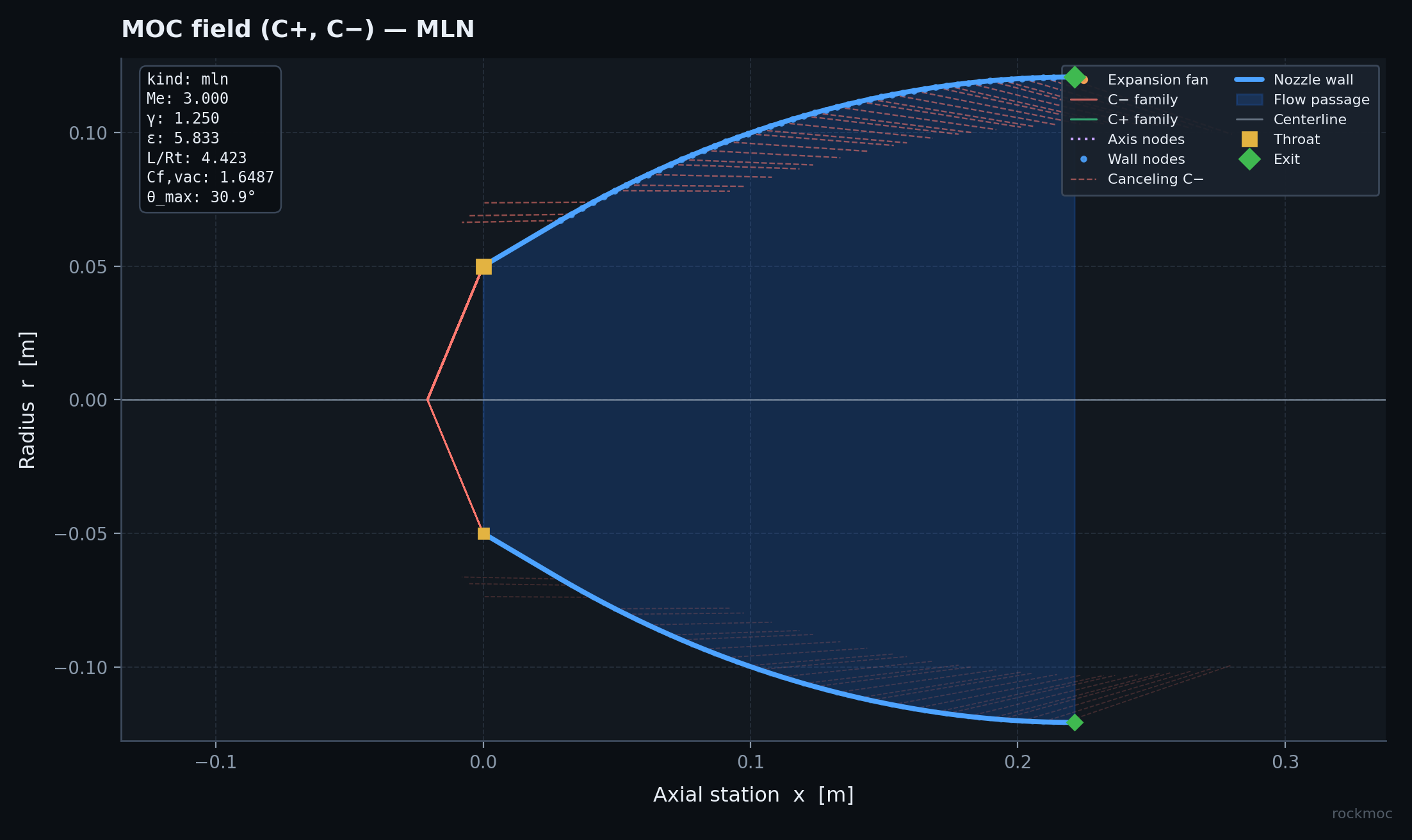
Sharp throat corner, expansion fan, canceling wall that tries to leave the exit nearly axial. Shortest contoured option when mass and length hurt. design_mln

Ideal / TIC

Ideal & truncated ideal

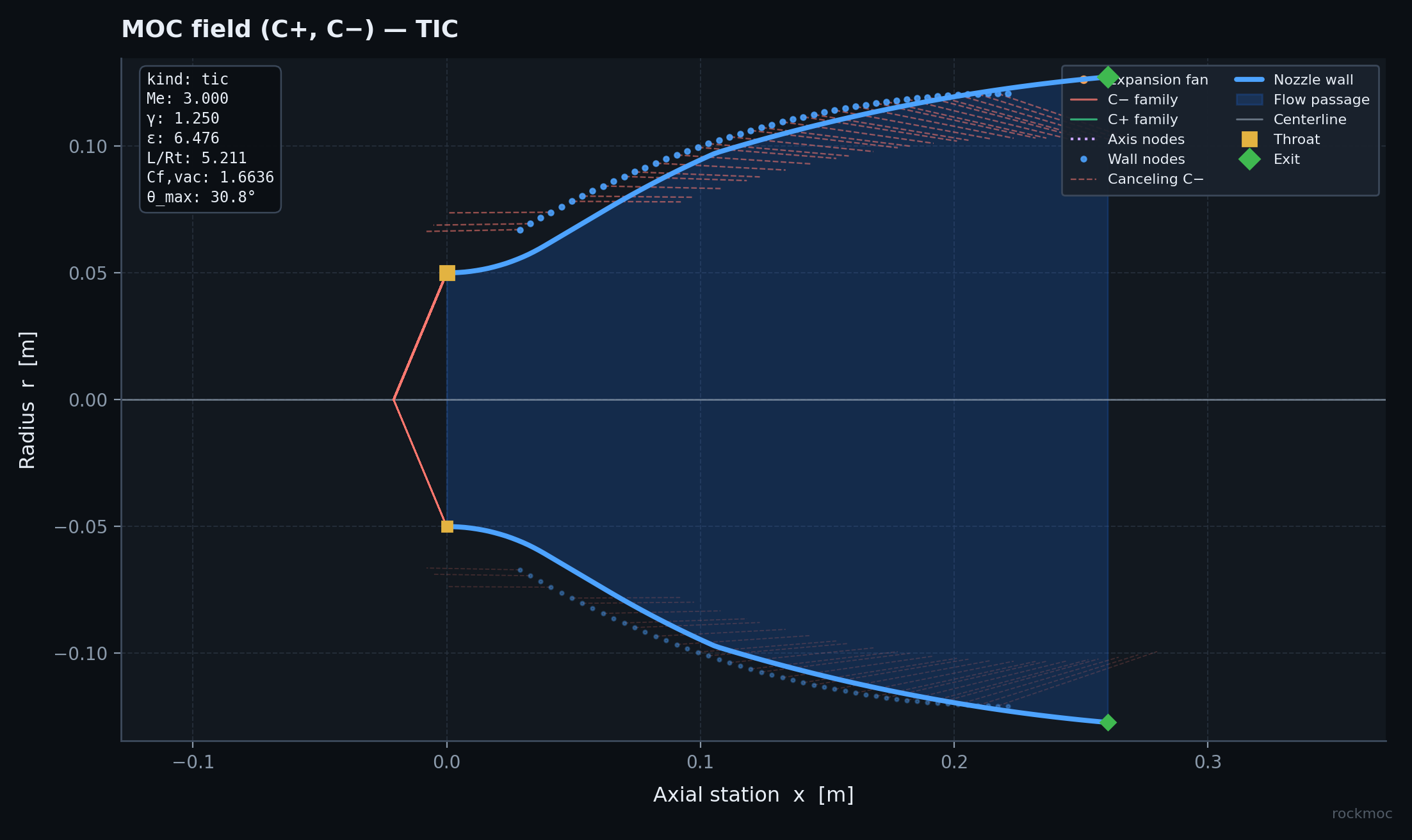
Circular-arc throat then a longer canceling region. TIC simply cuts that length (say 80%) when you cannot afford the full ideal bell. design_ideal · design_tic

Rao

TOP / TOC engineering bells

Thrust-oriented contours used in industry practice; length is a fraction of the equivalent 15° cone. Attachment angle sits above exit angle by design. design_rao

Cone

Conical baseline

Straight wall at a fixed half-angle (default 15°). Dead simple, easy to grade, and the right thing to beat before you claim “MOC is better.” design_conical

Planar NASA

TM-X-1502 sharp-throat MLN

Two-dimensional paper-faithful path: θ_max = ν_e/2 and exit height = A/A*. Great for labs that follow the NASA sample case. design_planar_mln_nasa

Spike

Annular aerospike

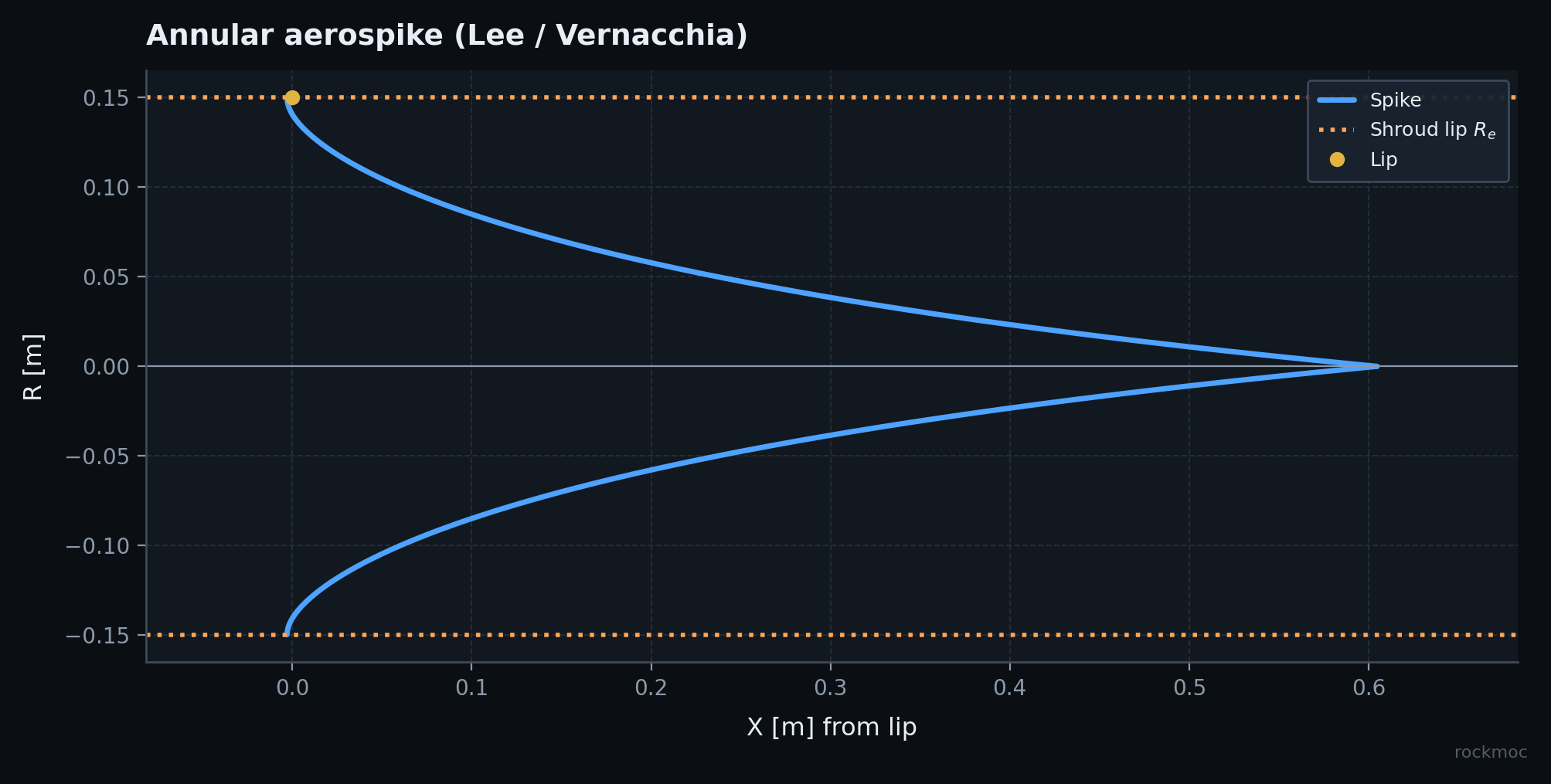
Lee/Vernacchia plug geometry with truncation, base pressure, and optional primary cowl — for altitude-compensation stories instead of closed bells. design_spike

Overlay of MLN, ideal, TIC and Rao walls

Family overlay

Same design point, four walls drawn together so the length trade is obvious.

Metric bars

L/R_t, area ratio, and vacuum C_F in one glance for a report figure.

Physics core

METHOD OF CHARACTERISTICS,
NOT A BLACK BOX

The solver marches along Mach waves the way Zucrow & Hoffman and NASA TM-X-1502 describe. You can inspect the net, not just the final polyline.

Wave directions in the meridional plane

(dr/dx)± = tan(θ ± μ) · μ = arcsin(1/M)

Axisymmetric geometric source (δ = 1)

d(θ ± ν)/dx = − sinθ · sinμ / (r · cos(θ ± μ))

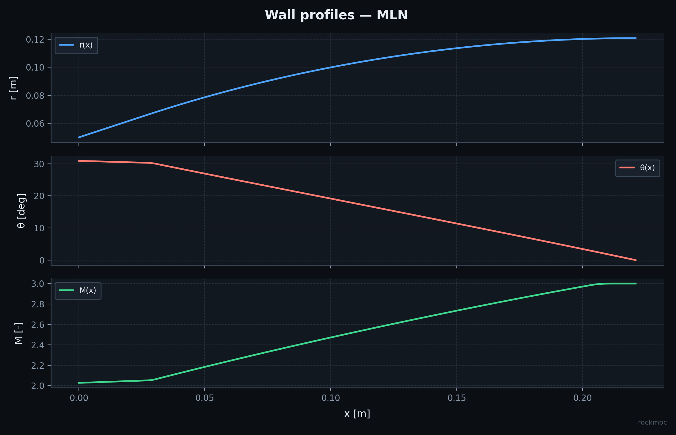
Interior points solve C− ∩ C+. The axis forces θ = 0. The canceling wall follows the classic MLN angle schedule and is scaled isotropically so geometric ε matches one-dimensional A/A*(M_e) without warping wall slopes.

THERMO YOU CAN CHECK

Area–Mach A/A* = f(M, γ)
Prandtl–Meyer ν(M) and its inverse
Isentropic pe/pc, temperatures, densities
Ideal vacuum / ambient thrust coefficient (Sutton form)
ν_max as M → ∞ from Shapiro’s closed form

Multi-γ tables let γ change with Mach for production runs. Chemistry backends only set better chamber γ, R, and T_c — they do not turn rockmoc into a reacting CFD code, and the docs say so out loud.

Wall contour

Mirrored passage, throat and exit markers, wall-angle color along the surface.

Profiles along x

Radius, wall angle, and edge Mach — the three numbers graders look for.

Production path

WHEN A SKETCH HAS TO BECOME A PACKAGE

design_production() is the “I need to hand this to CAD and still sleep” path.

01

FINE MOCdense mesh

02

γ TABLEperfect / multi-γ

03

THROATSauer IVL

04

BL δ*grow the wall

05

FIELD C_Fexit plane

06

ALTITUDEoff-design

07

UQmesh check

Boundary-layer add-on

Inviscid wall vs δ*-corrected wall — same spirit as NASA TM-X-2343.

Altitude package

How C_F and I_sp climb as ambient pressure falls.

Performance

NUMBERS YOU CAN DEFEND
IN A LAB REPORT

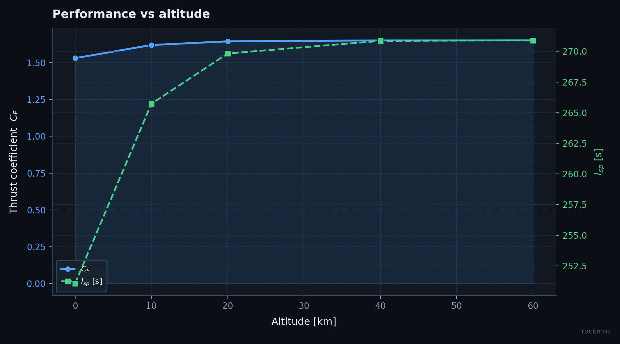
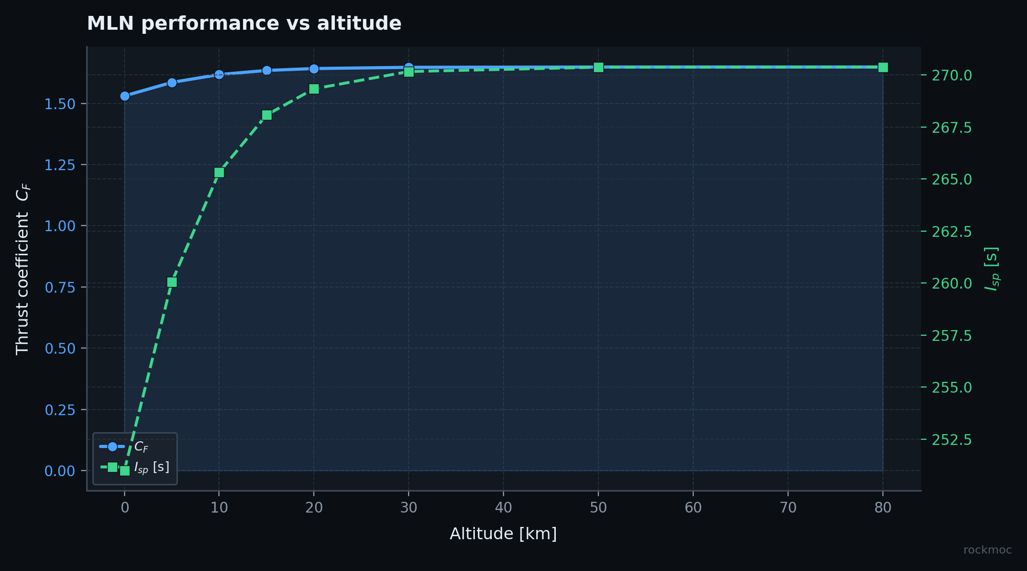
Vacuum C_F starts from classic isentropic formulas. Divergence losses use the exit angle, not a vague “wall looked curved so subtract 2%.” Field integration does the exit-plane momentum/pressure sum when you ask for it.

Altitude sweep

Sea level to near-vacuum for a fixed contour.

O/F sweep

How mixture ratio moves I_sp, C_F, γ, and ε together.

Area-ratio trade

Bigger ε buys vacuum performance — and length.

Edge Mach & p/p_c

Isentropic thermo glued to the wall mesh.

Gallery

FIGURES FROM THE ACTUAL SOLVER

Click any image to zoom. These are the same dark plots the library writes to disk.

MOC field

Fan, C+ / C− families, canceling rays, wall.

Contour

Metrics box + wall-angle color.

Wall profiles

r, θ, M along the axis.

γ sweep

How specific-heat ratio stretches the nozzle.

Ideal MOC

Longer canceling region than MLN.

TIC wall

Ideal family, cut short on purpose.

Rao TOP

Compact high-thrust engineering shape.

Ideal M–p

Edge thermo for the long bell.

Production MOC

Finer mesh on the production path.

BL correction

δ* grows the exit a little.

Altitude dashboard

Off-design package figure.

Production profiles

Full wall state for the package.

Aerospike contour

Annular spike with shroud lip radius marked.

Related MOC field

Truncated-family characteristics for comparison.

Interactive charts

THE SAME TABLES, ALIVE

Chart.js plots built from Anderson/NACA gold digits and the deep validation snapshot.

PRANDTL–MEYER ν(M) · γ = 1.4

Reference table digits vs rockmoc — errors sit well under a hundredth of a percent.

AREA RATIO A/A* · γ = 1.4

The same relation that sizes ε and planar exit height.

VALIDATION SNAPSHOT

43 cases · 170 metrics · 12 sources · zero failures on the deep campaign.

FAMILY LENGTH ORDER (Me = 3, γ = 1.25)

Illustrative L/R_t from a fair compare_nozzle_designs run (mesh changes absolute length a bit).

Validation

TWELVE SOURCES · FORTY-THREE CASES

Every deep-campaign metric stores reference, solver value, and error percent. Re-run anytime with py -3.12 tests/run_deep_validation.py.

43/43

Cases passed

170

Metrics checked

12

Cited sources

~0%

Median error

WHERE THE NUMBERS COME FROM

AndersonModern Compressible Flow — teaching tables for ν, A/A*, pe/pc at γ = 1.4

NACA Report 1135Ames (1953) — equations, tables, and charts for compressible flow

NASA TM-X-1502Vanco & Goldman (1968) — planar sharp-throat MLN computer program

NACA RM E8J12Shames & Seashore (1948) — 2D sharp-edge nozzle design data

NASA TM-X-2343Goldman & Vanco (1971) — MLN plus boundary-layer displacement

Rao 1958Exhaust nozzle contour for optimum thrust (TOP length practice)

Lee / VernacchiaAnnular aerospike; δ = π/2 − ν_e

Sutton & BiblarzRocket Propulsion Elements — ideal one-dimensional C_F

Zucrow & HoffmanGas Dynamics — axisymmetric MOC unit processes

Huzel & HuangLiquid rocket engine design — 15° conical nozzle baseline

Sauer / KliegelTransonic throat initial-value line for MOC starts

ShapiroCompressible fluid flow — Prandtl–Meyer form and ν_max

SAMPLE GOLD TABLE · γ = 1.4

M	ν ref°	ν solver	err %	A/A* ref	A/A* solver	err %
1.5	11.905	11.90521	0.0018	1.1762	1.17617	0.0028	PASS
2.0	26.380	26.37976	0.0009	1.6875	1.68750	~0	PASS
3.0	49.757	49.75735	0.0007	4.2346	4.23457	0.0008	PASS
4.0	65.785	65.78482	0.0003	10.7188	10.71875	0.0005	PASS
5.0	76.920	76.92022	0.0003	25.000	25.00000	~0	PASS

“If a code cannot hit Anderson’s ν(M=2) and NASA’s planar θ_max = ν_e/2, it has no business designing a flight contour.” — the bar rockmoc’s validation suite is written against

For students

BUILT FOR LABS, NOT JUST DEMOS

Homework should not fight the API. Defaults, reports, and docs are written for people learning propulsion.

Reports

Printable summaries

result.report(length_unit="mm") talks in mm and degrees. lab_report("lab.md") drops a checklist-ready Markdown skeleton.

Gases

Named teaching gases

example_gas("lox_rp1"), air, LOX/LH2, methalox — frozen estimates with a clear “not flight thermo” disclaimer.

Errors

Fix + example lines

Forgot that only one of Me / ε / pe/pc is allowed? The error tells you what to change and shows a working line.

Docs

Glossary & problems

Symbol sheet, mini-explainers per nozzle type, eight worked problems with solution sketches.

Notebooks

Four Jupyter paths

First MLN, family compare, altitude performance, NASA planar sample — open and run.

Defaults

DesignSpec.student

Throat in millimeters, n = 40, optional gas name. Fast enough for office hours.

from rockmoc import DesignSpec, design_mln, compare_nozzle_designs

spec = DesignSpec.student(Me=3.0, gas_name="lox_rp1", Rt_mm=50)
mln = design_mln(spec)
print(mln.report())
mln.lab_report("my_lab.md", student_name="Alex", course="AE-4XX")
print(compare_nozzle_designs(spec).to_markdown())

Architecture

WHERE THE CODE LIVES

Small, focused packages under src/rockmoc/ — easy to open one file and understand one idea.

thermo/

Gas models

Perfect gas, multi-γ tables, optional chemistry backends.

moc/

Characteristics

Unit processes, planar NASA, axisym HF, wall builders.

designers/

Nozzle builders

MLN, ideal, TIC, Rao, conical, production wrapper.

aerospike/

Plug nozzles

Lee spike, truncation, base pressure, cowl.

performance/

Metrics

1-D C_F, field integrals, altitude sweeps.

plot · student · validate

UX & proof

Dark figures, reports, literature campaign.

Get started

INSTALL · DESIGN · EXPORT

From a clone of the repo, editable install keeps you one edit away from experiments.

Install

pip install -e ".[plot,cli,dev]"
# optional chemistry stacks
pip install -e ".[cea]"
pip install -e ".[all]"

CLI

rockmoc design --type mln --Me 3.0 \
  --gamma 1.25 --Rt 0.05 -o wall.csv
rockmoc design --type tic --Me 4.0 \
  --truncate 0.8 -o tic.csv

Minimal design

from rockmoc import PerfectGas, DesignSpec, design_mln

gas = PerfectGas(gamma=1.25, R=350.0)
spec = DesignSpec(
    gas=gas,
    throat_radius=0.05,
    exit_mach=3.0,   # or area_ratio / pressure_ratio
    n_characteristics=80,
)
result = design_mln(spec, store_net=True)
print(result.summary())
result.export_csv("nozzle.csv")
result.plot()  # needs rockmoc[plot]

Call	What you get
`design_mln / ideal / tic / rao / conical`	Axisymmetric wall + metrics
`design_planar_mln_nasa`	NASA-style planar MLN
`design_spike*`	Aerospike family
`design_production`	Full accuracy package
`compare_nozzle_designs`	Family table (+ cone)
`run_deep_validation`	12-source campaign → JSON/CSV/MD

Honest limits

WHAT THIS IS NOT

Every report prints known limits so the tool is hard to misuse in a capstone.

Use it for

Homework, labs, design trades
Starting contours for CAD / CFD
Family comparisons and mesh studies
Teaching MOC with live figures

Do not treat it as

Shock / separation CFD
Multi-phase reacting flow
Heat transfer or structural FEA
Flight qualification without further analysis

A NOZZLE DESIGN LABIN A PYTHON PACKAGE